Macroeconomics Homework

Macroeconomics Homework

Seminar 2 + Homework

An individual anticipated that in the year 2000 his income would be 20 million out of which he plans a 2 million saving. Fortunately, he succeeds in earning 23 million and under these circumstances his savings reach the level of 3 million. Determine his marginal propensity to consume.

MPC= change in consumption/ change in disposable income = 3 / 23 = 0.13

We know that private consumption is illustrated by the relationship C=200+ 2/3*Yd. You are required to:

a.    determine the marginal propensity to consumption;

The consumption schedule demonstrates the relationship between income and consumption. MPC= dC/d(Yd), the derivative of C (consumption) with respect to Yd (disposable income). This derivative represents the change in C for every 1-unit change in Yd. The derivative of the ecuation for C, 200 +2/3 Yd, is 2/3. Therefore, MPC = 2/3 and every 1-unit (1 dollar) increase in disposable income causes an increase in consumption of 2/3 of a unit (67 cents). Since income is either saved or spent,

Disposable Income = Savings + Consumption

Yd = S + C

Yd = S + 200 + 2/3 Yd

b.   determine the marginal propensity to savings

The derivative of the savings equation, dS/d(Yd), is MPS = 1/3. This checks with the principle that income is either spent or saved; each additional dollar of disposable income is either spent or saved. Therefore MPC + MPS = 1 dollar, since each represents the fraction of the dollar that is either spent or saved.

1 - MPC = MPS = 1 - 2/3 = 1/3

c.    equation of savings function;

S= 1/3 Yd - 200

d.   Yd level corresponding to a zero level of savings (the break even level)

If disposable income is 600, savings is 1/3(600) - 200 = 200 - 200 =0. If Yd is less than 600, people will not be able to save; they will have to use up what they have already saved.

An economy is described by the following relationships: C=13+3/4Yd; T=4+0.2Y, I=10 and G=20. Fill in the table below with the corresponding levels of consumption, savings and the unplanned change in stocks. Then, based on this information determine the equilibrium level of income.

Explain the following function representing consumption (C) = 0,7 Y + 0,1 A, where Y and A represent the income level and the accumulated wealth. Demonstrate why the average propensity to consume is relatively constant on the long run.

Jack and Jill both obey the two-period Fisher model of consumption. Jack earns EUR 100 in the first period and EUR 100 in the second period, Jill earns nothing in the first period and EUR 210 in the second period. Both of them can borrow or lend at the interest rate r.

a)   You observe both Jack and Jill consuming EUR 100 in the first period and EUR 100 in the second What is the interest rate?

We can use Jill's intertemporal budget constraint to solve for the interest rate:

C1 + C2/(1+r) = Y1 + Y2/(1+r)

100+100/(1+r)=0+210(1+r)

100=110/(1+r)

r = 1.10

r = 0.10

b)   Suppose the interest rate increases. What will happen to Jack's consumption in the first period? Is Jack better off or worse off than before the interest rate rise?

The intertemporal budget constraint becomes steeper with the rise in the interest

rate. The opportunity cost of consuming today becomes larger. On other hand, the

overall income increase.

Jack is better off (reaches a higher indifference curve). This makes sense since his

purchasing power over both periods has increased (Y (1+r) has increased).

Note that the new budget constraint rotates around the (100,100) point, so we can

be sure that the substitution effect will dominate the income effect: That is,

consumption in period 1 will unambiguously decrease.

c)   What will happen to Jill's consumption in the first period when the interest rate increases? Is Jill better off or worse off than before the interest rate increase?

Note that it is different for Jill, who is forced to borrow in the first period (since

she has no income) in order to consume. [hence if c = 0 (horizontal axis); the

income equals y /(1+r) and if c = 0 (vertical axis), c = y ]. She becomes

necessarily worse off (both consumption today and tomorrow decrease)

Suppose an entrepreneur gets the opportunity to buy a machinery for 200 m.u. with a life-span of two years. The total revenue of his company will increase following this investment by 99 m.u. in the first year and by 121 m.u. in the second year. Would you recommend this investment, knowing that the interest rate to bank deposits is 12% when the inflation rate is 2%? Justify your answer.

Suppose the installment cost of a machinery with a life expectancy of 2 years is 200 m.u ; the revenue from this capital is 99 m.u in the first year and 121 m.u. in the second year. Is the company able to puchase this capital if the interest rate is 10

The inflation rate in one country was 13%. What would be the decision regarding a possible investment of 8 million knowing that it could bring a return of 9 million knowing that the reference interest rate is 12%?

A national economy is characterised by the following flows: C = 13 + ¾ Yd; T = 4 + 0,2 Y; I = 10; G = 20.

a) Fill in a table with the corresponding leves of Consumption (C), Savings (S) and unplanned investment stocks for the following levels of national income : 90; 100; 110.

b) How does the unemployment depend on output up to the equilibrium level? And beyond it? Explain.

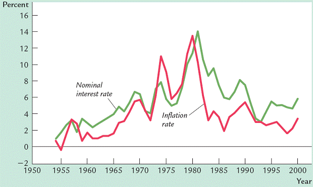
10. (Case Study) The graph below represents the evolution of the inflation rate (as measured by the CPI) and the nominal interest rate (expressed in three months Treasury bills) for US between 1950 and 2000. Explain the Fischer effect starting from this illustration.

Source: The Federal Reserve, the National Institute for Labor (from Mankiw&Taylor).

The effect proposes that if the real interest rate is equal to the nominal interest rate minus the expected inflation rate, and if the real interest rate were to be held constant, that the nominal rate and the inflation rate have to be adjusted on a one-for-one basis. Real interest rate = nominal interest rate - inflation rate. In simple terms: an increase in inflation will result in an increase in the nominal interest rate. For example, if the real interest rate is held at a constant 5.5% and inflation increased from 2% to 3%, the Fisher Effect indicates that the nominal interest rate would have to increase from 7.5% (5.5% real rate + 2% inflation rate) to 8.5% (5.5% real rate + 3% inflation rate).

11. Consider a closed simple economy with no state and foreign sectors. The data for consumption, income (production) and planned investment are as follows:

a.  Determine the Consumption function, the MPC (note that marginal propensity to consume is constant , between 0 and 1). Draw consumption as a function of income on a graph.

b. Determine the levels of savings and aggregate demand corresponding to each level of income;

c.  Determine the non-planned change in stocks and the current investment;

d. How will producers react if the income level is 150 billion? What if it is 400 billion?

e.  Determine the equilibrium level of income;

f.  How will a change of 5 billion in the planned investment affect the equilibrium level of income?

g. Represent on a graph the consumption and the aggregate demand functions. Draw the 45 degree line and compare the result with d.

h. Represent on the same graph savings as a function of income and the investment curve. Compare the results with the ones you obtained at point d.