Cancer Treatment using Magnetic Ablation

Cancer Treatment using Magnetic Ablation

Some types of cancerous tissue can be effectively treated by ablation using inductively heated ferromagnetic thermoseeds (Tompkins, 1992). The thermoseeds are surgically implanted into the tumor volume and heated inductively by exposure to an oscillating magnetic field. The thermoseeds can be made of an alloy having temperature-dependent magnetic properties so that the thermoseeds self-regulate their temperature. Above a critical temperature, the magnetic properties of the thermoseeds disappear and therefore they no longer absorb power from the magnetic field. Consequently, the thermoseeds provide internal generation at a rate that is sufficient to maintain the metal at the critical temperature but will not exceed the critical temperature. This problem will investigate the use of a cylindrical thermoseed placed within tumor tissue that is surrounded by normal tissue. This method of ablation was first introduced in EXAMPLE 1.3-1 and an analytical solution was obtained in the absence of blood perfusion. Magnetic ablation with blood perfusion was discussed in EXAMPLE 1.8-2. In general, an analytical solution to this problem is not possible because of the more complex two-dimensional geometry and the different properties of the tumor and the normal tissue, as shown in Figure 1.

Figure 1:

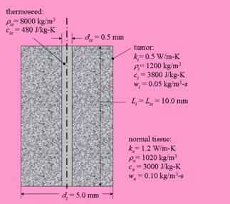The tumor is shaped as a cylinder with diameter d_t = 5.0 mm and length L_t = 10.0 mm. The conductivity, density and specific heat capacity of the tumor tissue are k_t = 0.5 W/m-K, r_t = 1200 kg/m³, and c_t = 3800 J/kg-K, respectively. Blood perfusion in the tumor is estimated to be w_t = 0.05 kg/m³-s. The tissue surrounding the tumor is normal liver with thermal conductivity, density and specific heat capacity k_n=1.2 W/m-K, r_n =1020 kg/m³ and c_n = 3000 J/kg-K. The rate of blood perfusion through the normal liver tissue is about double that of the tumor, w_n = 0.10 kg/m³-K. Normal body temperature (and blood temperature, for the perfusion term) is T_b =37°C. A single thermoseed is surgically implanted in the center of the tumor tissue. The thermoseed has diameter d_ts =0.5 mm and length L_ts =10 mm. As explained above, the properties of the thermoseed are such that it can be considered to be always at its critical temperature, T_crit, when the magnetic field exists. The density of the thermoseed alloy is r_ts =8000 kg/m³ and the specific heat capacity is c_ts =480 J/kg-K. The thermoseed is metallic and therefore has a very high conductivity.

The surgeon in charge of this procedure has indicated that the tumor tissue must be heated to a temperature of at least T_lethal =42°C over its entire volume during a 15 minute (900 sec) procedure. You are to determine the critical temperature of the thermoseed that will guarantee this result. It is also of interest to determine the maximum temperature within the normal tissue during the 900 sec heating process and the time required for the tissue to return to normal temperatures after the magnetic field is removed.

Start the FEHT program. A number of preparatory tasks must be done before the geometry can be specified. Since this problem involves blood perfusion, select Bio-Heat Transfer from the Subject menu to enable the bio-heat equation (Figure 2(a)). Select Cylindrical from the Setup menu to configure FEHT for cylindrical coordinates. Select Transient from the Setup menu since this problem will be time-dependent (Figure 2(b)).

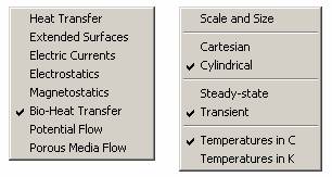
Figure 2: Menu settings used in (a) the Subject menu and (b) the Setup menu

Select Scale and Size from the Setup menu and set the scale, grid spacing and origin as shown in Figure 3. The parameters in Fig. 3 were selected to provide a grid with adequate resolution on the screen so that the geometry can be entered easily.

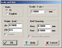
Figure 3: Scale and Size settings

Now it is necessary to describe the problem. When configured for cylindrical coordinates, FEHT expects only the objects that are on one side of the vertical center line (the line of symmetry). The centerline should be visible near the left edge of the screen. When materials overlap, as they do in this problem, FEHT requires the largest material to be drawn first. The largest material corresponds to the normal tissue. The exact dimensions of the normal tissue were not specified; however, it is only necessary to have the normal liver tissue to be much larger than the dimensions of the thermoseed so that the boundary conditions can be assumed to be at normal body temperature (37°C), unaffected by the existence of the thermal seed. Select Outline from the Draw menu and position the cursor on the center line near the left and top of the screen (e.g., at location R=0, Z=23 mm). Note that the coordinates of the cursor can be read at the upper left of the screen and that the grid lines are spaced 0.5 mm apart. Click to fix a node position on the center line. Move the cursor horizontally to a position that is 20 mm to the right of the center line and click to place the second node. Hold the Shift key down to ensure that the line drawn between your first and second nodal point will be horizontal. It is not important to position the this point exactly since the node can be moved later. Now move the cursor down vertically 20 mm and click to place a node at the lower right corner (e.g., R=20 mm, Z=3 mm). Again, hold the Shift key down to ensure that the line constructed between the nodes is vertical. Complete the process by moving horizontally back to the centerline and clicking and then vertically back to the initially point and clicking. 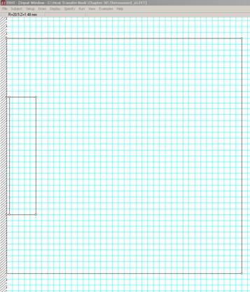Hold the Shift key down during this process. FEHT should acknowledge that the outline of the material is completed by flashing its boundary lines. The screen display should now appear as shown in Figure 4.

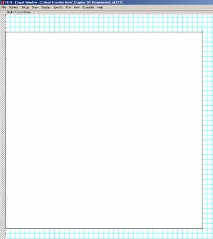
Figure 4: FEHT Input window showing outline of normal liver tissue

The node positions can now be set more exactly if desired. Select any of the four nodes by clicking on it. The node should flash. Now select the Node information menu item in the Specify menu (Figure 5). (As a short-cut, you can double-click on the node to bring up this dialog.). Exact values can now be specifed for the R and Z positions. Note that, depending on your screen resolution, it may not be possible to use to exact coordinates provided above; however, the exact positions of the nodes for the liver tissue are not important as long as it is large relative to the thermoseed and tumor. In this case, set the radius and height of the normal tissue near the limits of the screen.

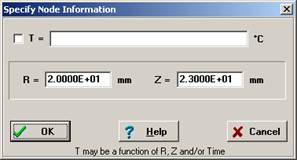
Figure 5: Node Information dialog

This drawing process is repeated for the tumor tissue. It may be helpful to select the Hide Patterns item from the Display menu so that the grid lines are not obscured. Select Outline from the Draw menu and click to place a node 5 mm below the top of the normal tissue. Holding the Shift key down, move the cursor 2.5 mm to the right and click to place the second node. Again, don't be concerned about the exact node position since you can move the node later. Move the cursor down (Shift key down) 10 mm and click. Finish the drawing by moving the node horizontally to the center line and clicking and then click on the first node. The outline of the tumor will flash.

Finally it is necessary to draw the thermoseed with the same height as the tumor tissue and a radius of 0.25 mm. FEHT internally checks where you attempt to position a nodes and it will not allow nodes to be placed such that the material boundaries cross. Unfortunately, it is sometimes overzealous in its checking. The easiest way to enter the thermoseed is as follows. Select the Outline command from the Draw menu. Move the cursor to the upper right position of the thermoseed which should be on the boundary between the tumor and normal tissue and 0.5 mm to the right of the centerline. This node should be located at a radius of 0.25 mm, not 0.5 mm, but if you try to place the node at 0.25 mm, it may jump to the node on the centerline. We will place it at 0.5 mm and move it later. Alternatively, the Zoom command could be applied to enlarge the drawing area which would prevent this problem. Click to position the node. Now move the cursor vertically down 10 mm (hold the Shift key down) and click to position the node on the existing tissue boundary. Finish the outline by moving horizontally and clicking on the centerline and then vertically, clicking on the first thermoseed node. Double-click on each node to set the positions so that the radius of the thermoseed is exactly 0.25 mm. At this point the screen should appear as seen in Figure 6.

Figure 6: FEHT Input window showing outline of the thermoseed and the normal and tumor tissue

Next, the properties of each material in the model must be specified. First, select Show Patterns from the Display menu so that the colors or patterns associated with each material type will be displayed. Double-click anywhere within the normal tissue outline. The Specify Properties dialog, shown in Figure 7, should appear. Liver should be one of the items shown in the list at the left. If so, click on it to select the properties for liver and enter a perfusion of 0.10 kg/m³-s. If Liver is not one of the default items, then select one of the 'not specified' options and enter the liver properties shown below.

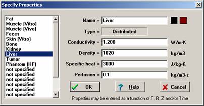
Figure 7: Property specifications for the normal liver tissue

Click OK to set the properties and dismiss the dialog. Next, double-click in the tumor tissue outline and set its properties, as shown in Figure 8.

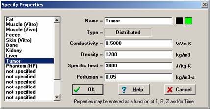
Figure 8: Property specifications for the tumor tissue

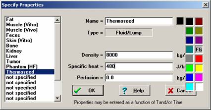
Finally, double-click in the thermoseed outline. There is no default material for the thermoseed. Click on a not specified item and enter the properties of the thermoseed, as shown in Figure 9. First enter the name, Thermoseed. Because it is made of high conductivity metal, the thermoseed will be at essentially a spatially uniform temperature; it is possible to either set a very large conductivity and allow FEHT to solve the governing partial differential equation, Eq , throughout the thermoseed region. However, this is a waste of computational resources given that we know that there are no significant temperature gradients within the thermoseed. However, FEHT allows you the option of specifying that a region is isothermal; this option is obtained by selecting Fluid/Lump from the Type list. Set the color pattern to gray to clicking in the second square box to the right of the name field.

.

Figure 9: Property specifications for the thermoseed

The boundary conditions should be set next. The boundaries that lie on the centerline are adiabatic by symmetry considerations. Move the mouse over one of the centerline boundaries and click. The line will flash to acknowledge that it is selected. Click on each of the centerline boundaries. When all three of them are flashing, select the Boundary Conditions menu item from the Specify menu and enter a heat flux of 0.0 W/m², as shown in Figure 10.

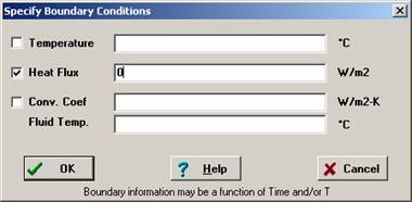
Figure 10: Adiabatic specification for centerline boundaries

Next, click on the top, right, and bottom boundaries of the normal tissue. It is assumed that these boundaries are far enough away from the thermoseed so that they are unaffected by the procedure and therefore these boundaries will be set to the normal body temperature, 37°C (Figure 11). The calculations, discussed subsequently, will show that this is a valid assumption.

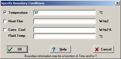
Figure 11: Constant temperature boundary for the normal tissue

There is one more set of boundary conditions that must be set and that is the boundaries between the thermoseed and the tumor and liver tissue. In this case, the boundary condition that must be specified is a convection coefficient; it is always necessary to specify a convection coefficient when a Lumped/Fluid element is used. Click on all three boundaries that surround the thermoseed and then select Boundary Conditions from the Specify menu (Figure 12). It may be difficult to select the small boundaries at the top and bottom of the thermoseed. If so, you can use the Zoom command to enlarge the display or drag a selection box around the thermoseed. (If the centerline boundary is also selected in this process, click on it to de-select it.) You may wish to Group these three boundaries after they are selected and flashing using the Group command in the Draw menu. When the boundaries are grouped, selecting any one will select all of the boundaries in the group so that it will be easy to change the boundary specification is necessary. Since there was no contact conductance listed in the problem statement, set a large convection coefficient, e.g., 10,000 W/m², to simulate essentially perfect thermal contact between the thermoseed and the tissue. The problem is now fully-specified. Save the file.

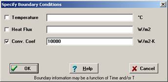
Figure 12: Boundary specification between the thermoseed and the tumor tissue

The final step in preparing the finite element solution is to set up the mesh; the mesh must consist of triangles and no mesh is required in the Lumped/Fluid material (i.e., you do not need to mesh the thermoseed). As discussed in Section 2.7, FEHT does not automatically generate a mesh. However, it will automatically refine an existing mesh and therefore all that is necessary is to set up a crude triangular mesh. This process is accomplished by selecting Element Lines from the Draw menu. Clicking at two separate locations will specify a mesh line; it is generally best to click on existing nodes. Clicking on locations that do not have a node will create a node, but this should only be done to ensure that the entire domain is broken into triangles. Do not be concerned about the mesh size at this point. You may want to hide the pattern using the command in the Display menu so that the grid lines are visible. A crude mesh is shown in Figure 13; other mesh choices would be equally valid.

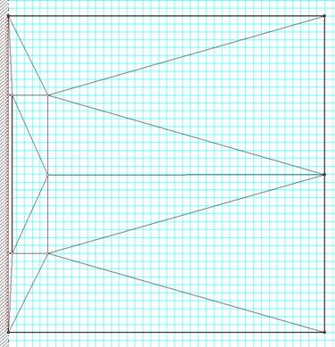
Figure 13: Input window showing the material outlines with a crude mesh

A final step is necessary for a transient problem; the initial conditions must be specified. Click anywhere within an outline of any material and then select the Initial Temperatures command from the Specify menu (Figure 14). Enter 37°C (normal body temperature) and click the check box to set the initial temperatures for all nodes in all three outlines to this initial temperature.

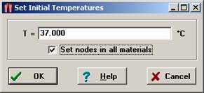
Figure 14: Specification of initial temperatures

Next, click on any point within the thermoseed and then select Lump Information from the Specify menu (Fig. 30-32). Enter the temperature for the thermoseed. This is the critical temperature of the alloy that we need to determine based on the surgical requirements. A reasonable first guess is 60°C. Save the file with a different name than you used last time.

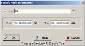
Figure 15: Specification of critical temperature for the thermoseed

The problem should now be ready to run. Select Calculate from the Run menu. You will be presented with a dialog (Figure 16) in which you enter the Stop and Step times. The Crank-Nicolson solution method is selected by default. As indicated in Section 3.2, this integration method is 3^rd order accurate and stable and therefore is much better suited for transient finite-element calculations than the alternatives. The Euler method choice is provided in FEHT only to demonstrate how much better the Crank-Nicolson method is for most problems. The option Do Nodal Balances is not selected by default. Nodal balances provide an accurate method of estimating energy rates from selected materials or material sections. Energy rates are not a concern in this problem, so nodal balances are not needed. Enter a stop time of 900 sec and a time step of 1 sec and then click the OK button.

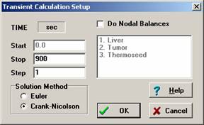
Figure 16: Specifications in the Calculate dialog

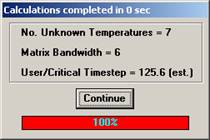
FEHT will run and then, if the calculations proceed without any problems, display a calculation summary (Figure 17).

Figure 17: Calculation summary for the crude mesh

The calculation summary shows the number of nodes that had undetermined temperatures (7) and the matrix bandwidth. The bandwidth is the largest number of nodes any one node is connected to, including itself. Many of the nodes shown in the crude mesh above are connected to 5 other nodes, resulting in the bandwidth of 6. Larger bandwidths require more computer effort. Finally, the ratio of the time step to the critical time step is shown. The critical time step is related to the Euler stability criterion discussed in Section 3.2.2.1. Using the Crank-Nicolson method, it is possible to take time steps that are much larger than the critical time step. Even a ratio of 125 may still result in an accurate solution. However, it will always be necessary to check the effect of time step by doing the calculations at progressively smaller time steps in order to see how the results are affected. The critical time step is affected by the mesh size so the time step may have to be reduced if the mesh is refined.

Several output display methods are now available. However, the mesh used to produce the results is very crude and the time step may be too large. Therefore, before the results are used to predict the required critical temperature it is necessary to reduce the mesh. Select Reduce Mesh from the Draw Menu. Select Calculate from the Run menu. Note that there are now 27 nodes and the ratio of the user to critical time step has increased to 500. FEHT does the calculations very quickly and the version of the program provided with this text will allow up to 1000 nodes. Reduce the mesh again and repeat the calculations, this time using 0.1 sec as the timestep; the output summary is shown in Figure 18. Save the file with a new name.

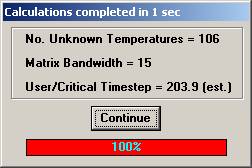
Figure 18: Calculation summary for the refined mesh with a 0.1 s timestep

Now it is useful to examine the calculation results. Select the Temperatures menu item from the View menu to show the temperatures at each node at the conclusion of the calculation, i.e. at time = 900 sec (Figure 19). The temperatures at the cursor location can be viewed in the left section of the status bar at the upper left of the screen by pressing the left mouse button.

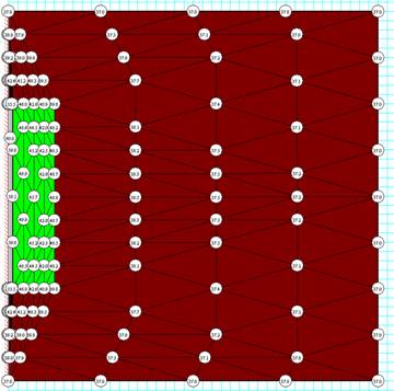
Figure 19: Calculated temperatures at each node at 900 sec

Note that the lowest temperature along the boundary between the tumor and normal tissue is about 40°C, a bit lower than 42°C required to kill the tumor. Note that the temperatures at any time during the process can also be viewed by selecting the Temperature Contours menu item in the View menu (Figure 20). A movie of the contours developing with time can be viewed by selecting the From Start to Stop option. Note that the minimum and maximum temperatures occurring during the selected time period are displayed at the upper left.

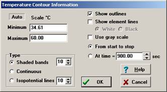
Figure 20: Temperature contour setting options

The minimum temperature is seen to be 34.6°C, which should be disturbing, since the minimum temperature in this problem should 37°C. This non-physical result tends to occur near the start of the transient process due to the use of the linear finite elements employed by FEHT. This behavior can be reduced by using shorter time steps, but it will not be possible to completely eliminate this effect because of the infinite temperature gradient that is imposed at time = 0 (the thermoseed has a temperature of 60°C while the surrounding tumor and tissue is initially at 37°C). Usually, only the first few time steps are affected. A plot of the temperatures at selected positions as a function of time demonstrates this behavior. To create this plot, select Input from the View menu to return to the drawing. Now click on the nodes for which you wish to know the temperature history. For example, click on all of the nodes that lie on the horizontal line along the middle of the domain and select the Temperatures vs Time menu item in the View menu. The plot shown in Figure 21 will be created showing the temperature of the selected nodes as a function of time.

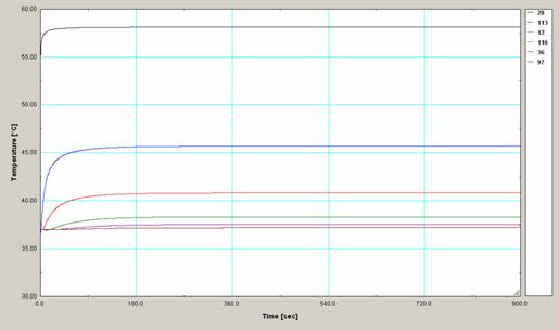
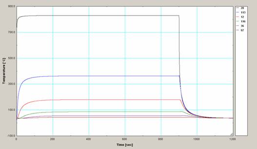
Figure 21: Temperature time history for nodes along a horizontal center line

Note that the temperatures at all of the selected locations reach their steady-state values quickly, within 90 sec or less. In the absence of blood perfusion, the heating associated with the thermoseed would not lead to a steady state; the influence of the thermoseed would continue to spread through the tissue, theoretically forever. However, Figure 22 shows that a steady-state is reached due to the effect of blood perfusion because energy will eventually be transported out of the tissue by the blood at the same rate that it is conducted in from the thermoseed.

No evidence of temperatures going below 37°C is evident in Figure 21. Further investigation reveals that the nodes that lie within the normal liver tissue just above and below the thermoseed exhibit this anomalous behavior. There are four nodes here, but they are so close together that they cannot easily be selected. Use the Zoom command to enlarge the display in this area; a rectangle will appear on the screen, click once to fix the location of the upper left corner of the rectangle and move the cursor to the lower right to enlarge the rectangle. The smaller the rectangle, the larger the magnification effect will be. Click to set the zoom (Figure 22).

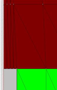
Figure 22: Zoomed view shown nodes above the thermoseed

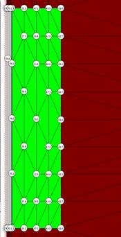
Now the four nodes above the thermoseed at the upper left corner of Figure 22 can be selected and their temperature history can be plotted. The non-physical effect associated with the temperature dropping below 37°C occurs very early in the calculations; double-click on the Time axis and set full scale to be 5 s so that the extent of the problem is visible (Figure 23). Notice that this problem will not have a significant effect on the results for times beyond 10 s.

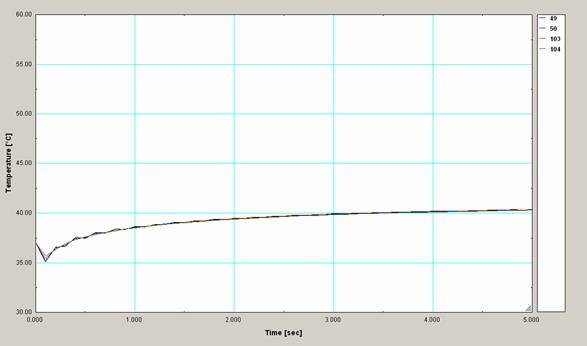
Figure 23: Time-temperature history for four nodes above the thermoseed showing non-physical results

It is tempting to accept the results obtained this far as being accurate. After all, they were obtained with a computer. However, there are many possible sources of error. Perhaps the mesh size and/or time step need to be reduced further. Save your file with a different name than last time, and then reduce this mesh. Run the calculations again with a 0.1 sec timestep. The node numbers are not affected by the mesh reduction process, so it is possible to compare the temperature time history for this reduced mesh with the results obtained before by plotting the temperatures of nodes 29, 113, 12, 116, 36, and 97 (i.e., the nodes shown in Figure 22) as a function of time and comparing the plot with Figure 21. The plots are virtually identical in this case indicating that the mesh is sufficiently refined. Reduce the time step to 0.01 sec and repeat the calculations. FEHT will have to do a large number of calculations to complete this process, so be patient. (The calculations required 84 sec on a 3.5 GHz machine.) A plot of the temperature-time history for the same six nodes shows no discernable differences. We can return to the previously saved file and continue further calculations using the mesh with 106 nodes and 0.1 s timesteps, now knowing that both the mesh and time steps are adequate for this problem.

The problem statement asked for the thermoseed critical temperature required to ensure that the boundary between the tumor and normal tissue attains a temperature of 42°C. The lowest temperatures (39.8°C at 900 sec) occur at the upper and lower right nodes of the tumor. With some experimentation, it can be found that a 78°C thermoseed is necessary in order to meet this criterion. The resulting temperature distribution is shown in Figure 24. The results in this figure also show that portions of the normal liver tissue will be heated to temperatures significantly higher than 42°C. The highest temperatures occur in the vicinity of the thermoseed. It is likely that this normal tissue will be killed, along with the tumor tissue. Using a shorter thermoseed that does not extend over the complete length of the tumor could perhaps reduce the undesirable effect.

Figure 24: Zoomed view showing final calculated temperature at nodes in the tumor

Additional studies can now be conducted. For example, it is of interest to know how long it will take to for the temperatures in the tissue to return to normal body temperature after the magnetic field is removed. To do this study, first click on Input in the View menu to return to the drawing input window. Click within the thermoseed and then select Lump Information from the Specify menu. Uncheck the box that fixed the temperature of the lump to the critical temperature. Now, the thermoseed temperature will be calculated based on conduction with the tumor tissue that it contacts. The initial conditions for this calculation are the temperatures that existed at 900 sec from the previous calculation. FEHT will set these initial conditions when you select Continue (rather than Calculate) from the Run menu. Enter a stop time of 1200 sec. The temperature-time history for the nodes along a horizontal center line in Figure 25 show that the tissue returns to normal temperature within 100 sec after the magnetic field is turned off.

Figure 25: Temperature time history showing the period after the magnetic field is removed