Introduction to Predictive Modeling: Regressions

Introduction

Regressions offer a different approach to prediction compared to decision trees. Regressions, as parametric models, assume a specific association structure between inputs and target. By contrast, trees, as predictive algorithms, do not assume any association structure; they simply seek to isolate concentrations of cases with like-valued target measurements.

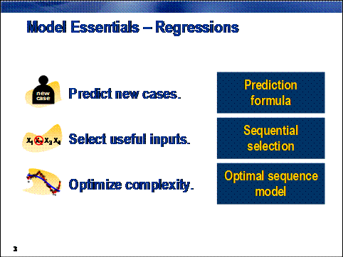
The regression approach to the model essentials in SAS Enterprise Miner is outlined over the following pages. Cases are scored using a simple mathematical prediction formula. One of several heuristic sequential selection techniques is used to pick from a collection of possible inputs and creates a series of models with increasing complexity. Fit statistics calculated from validation data select the optimal sequence model.

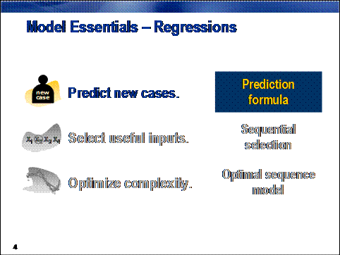
Regressions predict cases using a mathematical equation involving values of the input variables.

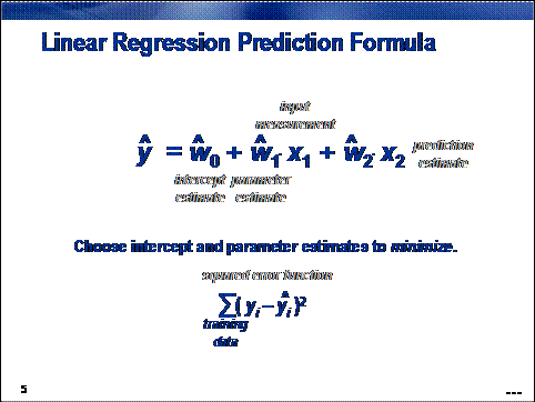
In standard linear regression, a prediction estimate for the target variable is formed from a simple linear combination of the inputs. The intercept centers the range of predictions, and the remaining parameter estimates determine the trend strength (or slope) between each input and the target. The simple structure of the model forces changes in predicted values to occur in only a single direction (a vector in the space of inputs with elements equal to the parameter estimates).

Intercept and parameter estimates are chosen to minimize the squared error between the predicted and observed target values (least squares estimation). The prediction estimates can be viewed as a linear approximation to the expected (average) value of a target conditioned on observed input values.

Linear regressions are usually deployed for targets with an interval measurement scale.

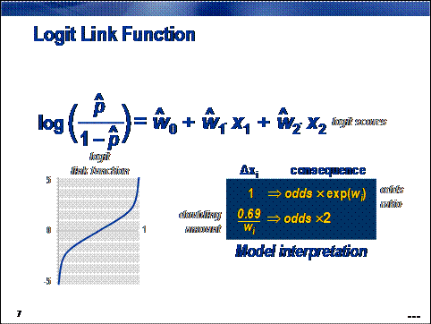
Logistic regressions are closely related to linear regressions. In logistic regression, the expected value of the target is transformed by a link function to restrict its value to the unit interval. In this way, model predictions can be viewed as primary outcome probabilities. A linear combination of the inputs generates a logit score, the log of the odds of primary outcome, in contrast to the linear regression's direct prediction of the target.

The presence of the link function complicates parameter estimation. Least squares estimation is abandoned in favor of maximum likelihood estimation. The likelihood function is the joint probability density of the data treated as a function of the parameters. The maximum likelihood estimates the values of the parameters that maximize the probability of obtaining the training sample.

If your interest is ranking predictions, linear and logistic regressions will yield virtually identical results.

For binary prediction, any monotonic function that maps the unit interval to the real number line can be considered as a link. The logit link function is one of the most common. Its popularity is due, in part, to the interpretability of the model.

There are two equivalent ways to interpret a logistic regression model. Both relate changes in input measurements to changes in odds of primary outcome.

An odds ratio expresses the increase in primary outcome odds associated with a unit change in an input. It is obtained by exponentiating the parameter estimate of the input of interest.

A doubling amount gives the amount of change required for doubling the primary outcome odds. It is equal to log(2) ≈ 0.69 divided by the parameter estimate of the input of interest.

If the predicted logit scores remain in the range -2 to +2, linear and logistic regression models of binary targets are virtually indistinguishable. Balanced sampling (Chapter 7) often ensures this. Thus, the prevalence of balanced sampling in predictive modeling might, in fact, be a vestigial practice from a time when maximum likelihood estimation was computationally extravagant.

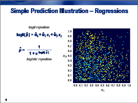
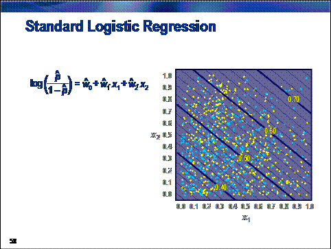
To demonstrate the properties of a logistic regression model, consider the two-color prediction problem introduced in Chapter 3. As before, the goal is to predict the target color, based on location in the unit square.

The predictions can be decisions, rankings, or estimates. The logit equation produces a ranking or logit score. To get a decision, you need a threshold. The easiest way to get a meaningful threshold is to convert the prediction ranking to a prediction estimate. You can obtain a prediction estimate using a straightforward transformation of the logit score, the logistic function. The logistic function is simply the inverse of the logit function.

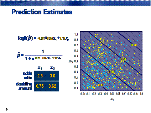
Parameter estimates are obtained by maximum likelihood estimation. These estimates can be used in the logit and logistic equations to obtain predictions. The plot on the right shows the prediction estimates from the logistic equation. One of the attractions of a standard logistic regression model is the simplicity of its predictions. The contours are simple straight lines. (In higher dimensions, they would be hyperplanes.) This enables a straightforward interpretation of the model using the odds ratios and doubling amounts shown at the bottom left. Unfortunately, simplicity can also lead to prediction bias (as scrutiny of the prediction contours suggests).

The last section of this chapter shows a way to extend the capabilities of logistic regression to address this possible bias.

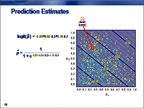
To score a new case, the values of the inputs are plugged into the logit or logistic equation.

This action creates a logit score or prediction estimate. Typically, if the prediction estimate is greater than 0.5 (or equivalently, the logit score is positive), cases are usually classified to the primary outcome. (This assumes an equal misclassification cost. See Chapter 7.)

While the prediction formula would seem to be the final word in scoring a new case with a regression model, there are actually several additional issues that must be addressed.

What should be done when one of the input values used in the prediction formula is missing? You might be tempted to simply treat the missing value as zero and skip the term involving the missing value. While this approach can generate a prediction, this prediction is usually biased beyond reason.

How do you score cases with unusual values? Regression models make their best predictions for cases near the centers of the input distributions. If an input can have (on rare occasion) extreme or outlying values, the regression should respond appropriately.

What value should be used in the prediction formula when the input is not a number? Categorical inputs are common in predictive modeling. They did not present a problem for the rule-based predictions of decision trees, but regression predictions come from algebraic formulas that require numeric inputs. (You cannot multiply marital status by a number.) A method to include nonnumeric data in regression is needed.

What happens when the relationship between the inputs and the target (or rather logit of the target) is not a straight line? It is preferable to be able to build regression models in the presence of nonlinear (and even non-additive) input target associations.

The above questions are presented as scoring-related issues. They are also problems for model construction. (Maximum likelihood estimation requires iteratively scoring the training data.) The first of these, handling missing values, is dealt with immediately. The remaining issues are addressed, in turn, at the end of this chapter.

The default method for treating missing values in most regression tools in SAS Enterprise Miner is complete-case analysis. In complete-case analysis, only those cases without any missing values are used in the analysis.

Even a smattering of missing values can cause an enormous loss of data in high dimensions. For instance, suppose that each of the k input variables is missing at random with probability a. In this situation, the expected proportion of complete cases is as follows:

Therefore, a 1% probability of missing (a=.01) for 100 inputs leaves only 37% of the data for analysis, 200 leaves 13%, and 400 leaves 2%. If the missingness were increased to 5% (a=.05), then <1% of the data would be available with 100 inputs.

The purpose of predictive modeling is scoring new cases. How would a model built on the complete cases score a new case if it had a missing value? To decline to score new incomplete cases would be practical only if there were a very small number of missing values.

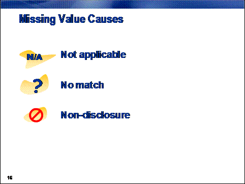
Missing values arise for a variety of reasons. For example, the time since last donation to a card campaign is meaningless if someone did not donate to a card campaign. In the PVA97NK data set, several demographic inputs have missing values in unison. The probable cause was no address match for the donor. Finally, certain information, such as an individual's total wealth, is closely guarded and is often not disclosed.

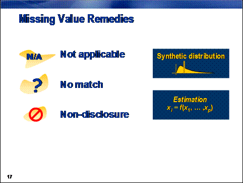
Missing value replacement strategies fall into one of two categories.

Synthetic distribution methods use a one-size-fits-all approach to handle missing values. Any case with a missing input measurement has the missing value replaced with a fixed number. The net effect is to modify an input's distribution to include a point mass at the selected fixed number. The location of the point mass in synthetic distribution methods is not arbitrary. Ideally, it should be chosen to have minimal impact on the magnitude of an input's association with the target. With many modeling methods, this can be achieved by locating the point mass at the input's mean value.

Estimation methods eschew the one-size-fits-all approach and provide tailored imputations for each case with missing values. This is done by viewing the missing value problem as a prediction problem. That is, you can train a model to predict an input's value from other inputs. Then, when an input's value is unknown, you can use this model to predict or estimate the unknown missing value. This approach is best suited for missing values that result from a lack of knowledge, that is, no-match or non-disclosure, but it is not appropriate for not-applicable missing values. (An exercise at the end of this chapter demonstrates using decision trees to estimate missing values.)

Because predicted response might be different for cases with a missing input value, a binary imputation indicator variable is often added to the training data. Adding this variable enables a model to adjust its predictions in the situation where missingness itself is correlated with the target.

Managing Missing Values

The demonstrations in this chapter assume that you completed the demonstrations in Section 4.1.

As discussed above, regression requires that a case have a complete set of input values for both training and scoring.

Right-click the PVA97NK data source and select Explore . from the menu. The
Explore - AAEM.PVA97NK window opens.

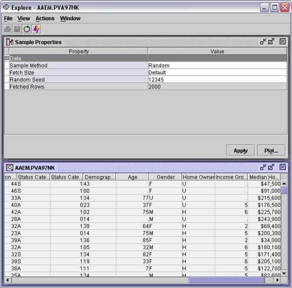
There are several inputs with a noticeable frequency of missing values, for example, Age and Income Group

There are several ways to proceed:

Do nothing. If there are very few cases with missing values, this is a viable option. The difficulty with this approach comes when the model must predict a new case that contains a missing value. Omitting the missing term from the parametric equation usually produces an extremely biased prediction.

Impute a synthetic value for the missing value. For example, if an interval input contains a missing value, replace the missing value with the mean of the non-missing values for the input. This eliminates the incomplete case problem but modifies the input's distribution. This can bias the model predictions.

Making the missing value imputation process part of the modeling process allays the modified distribution concern. Any modifications made to the training data are also made to the validation data and the remainder of the modeling population. A model trained with the modified training data will not be biased if the same modifications are made to any other data set that the model might encounter (and the data has a similar pattern of missing values).

Create a missing indicator for each input in the data set. Cases often contain missing values for a reason. If the reason for the missing value is in some way related to the target variable, useful predictive information is lost.

The missing indicator is 1 when the corresponding input is missing and 0 otherwise. Each missing indicator becomes an input to the model. This enables modeling of the association between the target and a missing value on an input.

To address missing values in the PVA97NK data set, impute synthetic data values and create missing value indicators.

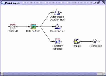
Select the Modify tab.

Drag an Impute tool into the diagram workspace.

Connect the Data Partition node to the Impute node.

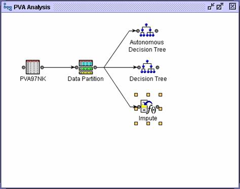
Select the Impute node and examine the Properties panel.

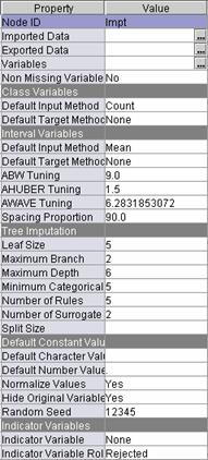
The defaults of the Impute node are as follows:

For interval inputs, replace any missing values with the mean of the non-missing value

For categorical inputs, replace any missing values with the most frequent category.

Select Indicator Variable Unique.

Select Indicator Variable Role Input.

With these settings, each input with missing values generates a new input. The new input named IMP_original_input_name will have missing values replaced by a synthetic value and nonmissing values copied from the original input. In addition, new inputs named M_original_input_name will be added to the training data to indicate the synthetic data values.

Run the Impute node and review the Results window. Three inputs had missing values.

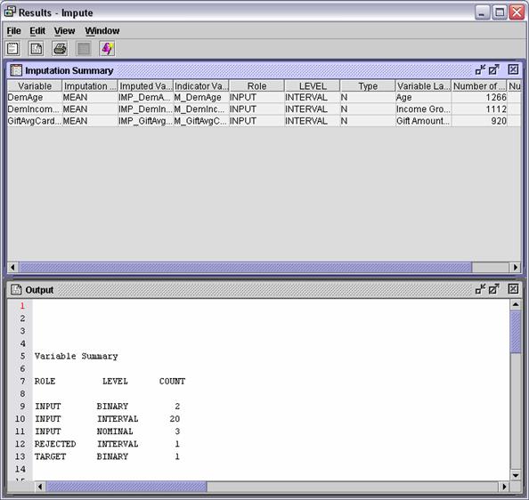
With all missing values imputed, the entire training data set is available for building the logistic regression model. In addition, a method is in place for scoring new cases with missing values. (See Chapter 8.)

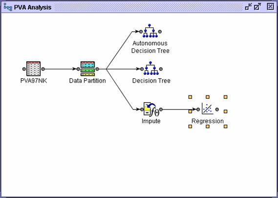
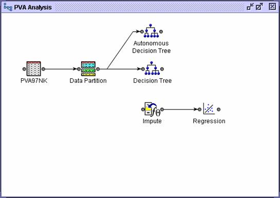
Running the Regression Node

There are several tools in SAS Enterprise Miner to fit regression or regression-like models. By far, the most commonly used (and, arguably, the most useful) is the simply named Regression tool.

Select the Model tab.

Drag a Regression tool into the diagram workspace.

Connect the Impute node to the Regression node.

The Regression node can create several types of regression models, including linear and logistic. The type of default regression type is determined by the target's measurement level.

Run the Regression node and view the results. The Results - Regression window opens.

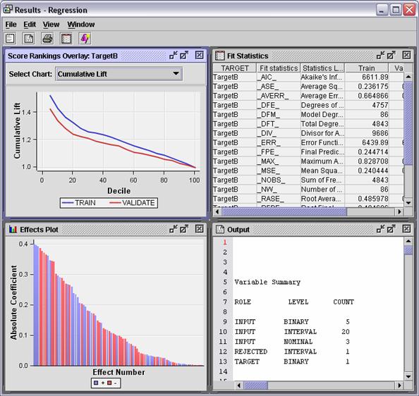
Maximize the Output window.

Lines 5-13 of the Output window summarize the roles of variables used (or not) by the Regression node.

The fit model has 28 inputs that predict a binary target.

Lines 45-57 give more information about the model, including the training data set name, target variable name, number of target categories, and most importantly, the number of model parameters.

Based on the introductory material on logistic regression that is presented above, you might expect to have a number of model parameters equal to the number of input variables. This ignores the fact that a single nominal input (for example, DemCluster) can generate scores of model parameters. You can see the number of parameters (or degrees of freedom) that each input contributes to the model, as well as each input's statistical significance, by viewing lines 117-146 of the Output window.

The Type 3 Analysis tests the statistical significance of adding the indicated input to a model that already contains other listed inputs. Roughly speaking, a value near 0 in the Pr > Chi-Square column indicates a significant input; a value near 1 indicates an extraneous input.

The statistical significance measures range from <0.0001 (highly significant) to 0.9997 (highly dubious). Results such as this suggest that certain inputs can be dropped without affecting the predictive prowess of the model.

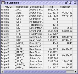
Restore the Output window to its original size and maximize the Fit Statistics window.

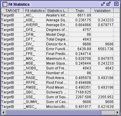
If the decision predictions are of interest, model fit can be judged by misclassification. If estimate predictions are the focus, model fit can be assessed by average square error. There appears to be some discrepancy between the values of these two statistics on the train and validation data. This indicates possible overfit of the model. It can be mitigated by employing an input selection procedure.

Selecting Regression Inputs

The second task that all predictive models should perform is input selection. One way to find the optimal set of inputs for a regression is simply to try every combination. Unfortunately, the number of models to consider using this approach increases exponentially in the number of available inputs. Such an exhaustive search is impractical for realistic prediction problems.

An alternative to the exhaustive search is to restrict the search to a sequence of improving models. While this might not find the single best model, it is commonly used to find models with good predictive performance. The Regression node in SAS Enterprise Miner provides three sequential selection methods.

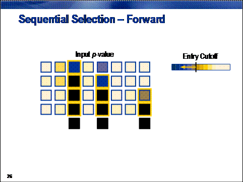
Forward selection creates a sequence of models of increasing complexity. The sequence starts with the baseline model, a model predicting the overall average target value for all cases. The algorithm searches the set of one-input models and selects the model that most improves upon the baseline model. It then searches the set of two-input models that contain the input selected in the previous step and selects the model showing the most significant improvement. By adding a new input to those selected in the previous step, a nested sequence of increasingly complex models is generated. The sequence terminates when no significant improvement can be made.

Improvement is quantified by the usual statistical measure of significance, the p-value. Adding terms in this nested fashion always increases a model's overall fit statistic. By calculating the change in the fit statistic and assuming that the change conforms to a chi-squared distribution, a significance probability, or p-value, can be calculated. A large fit statistic change (corresponding to a large chi-squared value) is unlikely due to chance. Therefore, a small p-value indicates a significant improvement. When no p-value is below a predetermined entry cutoff, the forward selection procedure terminates.

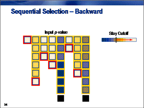
In contrast to forward selection, backward selection creates a sequence of models of decreasing complexity. The sequence starts with a saturated model, which is a model that contains all available inputs and, therefore, has the highest possible fit statistic. Inputs are sequentially removed from the model. At each step, the input chosen for removal least reduces the overall model fit statistic. This is equivalent to removing the input with the highest p-value. The sequence terminates when all remaining inputs have a
p-value in excess of the predetermined stay cutoff.

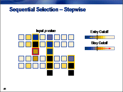
Stepwise selection combines elements from both the forward and backward selection procedures. The method begins in the same way as the forward procedure, sequentially adding inputs with the smallest p‑value below the entry cutoff. After each input is added, however, the algorithm re-evaluates the statistical significance of all included inputs. If the p-value of any of the included input exceeds a stay cutoff, the input is removed from the model and re-entered into the pool of inputs that are available for inclusion in a subsequent step. The process terminates when all inputs available for inclusion in the model have p-values in excess of the entry cutoff and all inputs already included in the model have p-values below the stay cutoff.

Selecting Inputs

Implementing a sequential selection method in the regression node requires a minor change to the Regression node settings.

Close the Regression results window.

Select Selection Model Stepwise on the Regression node property sheet.

The Regression node is now configured to use stepwise selection to choose inputs for the model.

Run the Regression node and view the results.

Select the Output tab and scroll to lines 95-121.

The stepwise procedure starts with Step 0, an intercept-only regression model. The value of the intercept parameter is chosen so that the model predicts the overall target mean for every case. The parameter estimate and the training data target measurements are combined in an objective function. The objective function is determined by the model form and the error distribution of the target. The value of the objective function for the intercept-only model is compared to the values obtained in subsequent steps for more complex models. A large decrease in the objective function for the more complex model indicates a significantly better model.

Step 1 adds one input to the intercept-only model. The input and corresponding parameter are chosen to produce the largest decrease in the objective function. To estimate the values of the model parameters, the modeling algorithm makes an initial guess for their values. The initial guess is combined with the training data measurements in the objective function. Based on statistical theory, the objective function is assumed to take its minimum value at the correct estimate for the parameters. The algorithm decides whether changing the values of the initial parameter estimates can decrease the value of objective function. If so, the parameter estimates are changed to decrease the value of the objective function and the process iterates. The algorithm continues iterating until changes in the parameter estimates fail to substantially decrease the value of the objective function.

The Step 1 optimization is summarized in the Output window, lines 121-164.

The output next compares the model fit in step 1 with the model fit in step 0. The objective functions of both models are multiplied by 2 and differenced. The difference is assumed to have a chi-square distribution with 1 degree of freedom. The hypothesis that the two models are identical is tested. A large value for the chi-square statistic makes this hypothesis unlikely.

The hypothesis test is summarized in lines 167-173.

Next, the output summarizes an analysis of the statistical significance of individual model effects (lines 176-181). For the one input model, this is similar to the global significance test above.

Finally, an analysis of individual parameter estimates is made. The standardized estimates and the odds ratios merit special attention.

The standardized estimates present the effect of the input on the log-odds of donation. The values are standardized to be independent of the input's unit of measure. This provides a means of ranking the importance of inputs in the model.

The odds ratio estimates indicate by what factor the odds of donation increase for each unit change in the associated input. Combined with knowledge of the range of the input, this provides an excellent way to judge the practical (as opposed to the statistical) importance of an input in the model.

The stepwise selection process continues for seven steps. After the eighth step, neither adding nor removing inputs from the model significantly changes the model fit statistic. At this point the Output window provides a summary of the stepwise procedure. The summary shows the step in which each input was added and the statistical significance of each input in the final eight-input model (lines 810-825).

The default selection criterion selects the model from step 8 as the model with optimal complexity (lines 828-830). As the next section shows, this might not be the optimal based on the fit statistic that is appropriate for your analysis objective.

For convenience, the output from step 9 is repeated. An excerpt from the analysis of individual parameter estimates is shown below (lines 857-870).

The parameter with the largest standardized estimate is GiftCntCard36

The odds ratio estimates show that a unit change in M_GiftAvgCard36 produces the largest change in the donation odds.

Restore the Output window and maximize the Fit Statistics window.

Considering the analysis from an estimate prediction perspective, the simpler stepwise selection model, with a lower validation average squared error, is an improvement over the full model (from the previous section). From a decision prediction perspective, however, the larger full model, with a slightly lower misclassification, is preferred.

This somewhat ambiguous result comes from a lack of complexity optimization, by default, in the Regression node. This oversight is handled in the next demonstration.

Optimizing Regression Complexity

Regression complexity is optimized by choosing the optimal model in the sequential selection sequence.

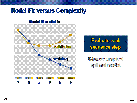
The process involves two steps. First, fit statistics are calculated for the models generated in each step of the selection process using both the training and validation data sets.

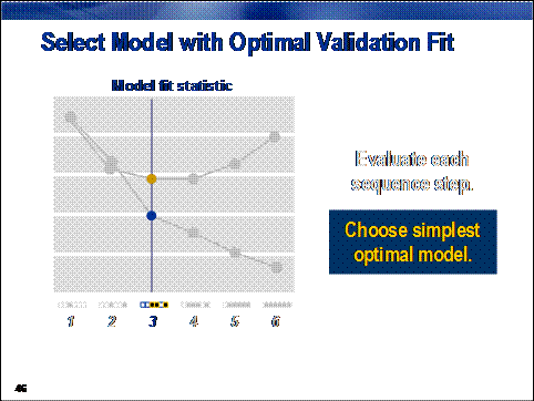
Then, as with the decision tree in Chapter 4, the simplest model (that is, the one with the fewest inputs) with the optimal fit statistic is selected.

Optimizing Complexity

In the same manner as the decision tree, you can tune a regression model to give optimal performance on the validation data. The basic idea involves calculating a fit statistic for each step in the input selection procedure and selecting the step (and corresponding model) with the optimal fit statistic value. To avoid bias, of course, the fit statistic should be calculated on the validation data set.

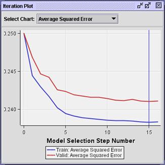
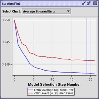
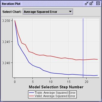
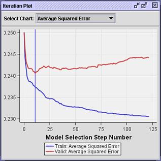
Select View Model Iteration Plot. The Iteration Plot window opens.

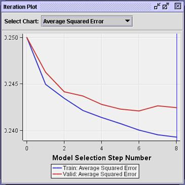
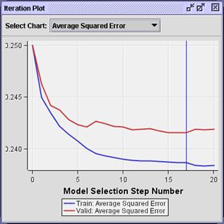
The Iteration Plot window shows (by default) the average squared error from the model selected in each step of the stepwise selection process. Apparently, the smallest average squared error occurs in step 6, rather than in the final model, step 8. If your analysis objective requires estimates predictions, the model from step 6 should provide slightly less biased ones.

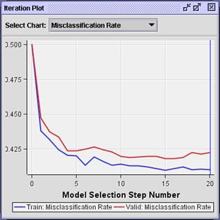
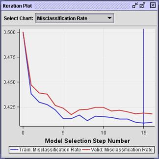
Select Select Chart Misclassification Rate.

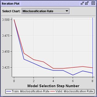
The iteration plot shows that the model with the smallest misclassification rate occurs in step 4. If your analysis objective requires decision predictions, the predictions from the step 4 model will be as accurate as the predictions from the final step 8 model.

The selection process stopped at step 8 to limit the amount of time spent running the stepwise selection procedure. In step 8, no more inputs had a chi-squared p-value below 0.05. The value 0.05 is a somewhat arbitrary holdover from the days of statistical tables. With the validation data available to gauge overfitting, it is possible to eliminate this restriction and obtain a richer pool of models to consider.

Close the Results - Regression window.

Select Use Selection Default No from the Regression node Properties panel.

Type in the Entry Significance Level field.

Type in the Stay Significance Level field.

The Entry Significance value enables any input into the model. (The one chosen will have the smallest p-value.) The Stay Significance value keeps any input in the model with a p-value less than 0.5. This second choice is somewhat arbitrary. A smaller value can terminate the stepwise selection process earlier, while a larger value can maintain it longer. A Stay Significance of 1.0 forces stepwise to behave in the manner of a forward selection.

Run the Regression node and view the results.

Select View Model Iteration Plot. The Iteration Plot window opens.

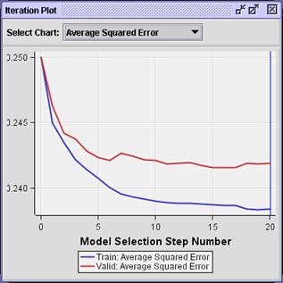
The iteration plot shows the smallest average squared errors occurring in steps 15 or 16.

Select Select Chart Misclassification Rate.

The iteration plot shows the smallest validation misclassification rates also occurring near steps 15-16.

You can configure the Regression node to select the model with the smallest fit statistic (rather than the final stepwise selection iteration). This method is how SAS Enterprise Miner optimizes complexity for regression models.

Close the Results - Regression window.

If your predictions are decisions, use the following setting:

Select Selection Criterion Validation Misclassification. (Equivalently, you can select
Validation Profit / Loss. The equivalence is demonstrated in Chapter 7.)

If your predictions are estimates (or rankings), use the following setting:

Select Selection Criterion Validation Error.

The continuing demonstration assumes validation error selection criteria.

Run the Regression node and view the results.

Select View Model Iteration Plot.

The vertical blue line shows the model with the optimal validation average squared error (step 17).

Select the Output window and view lines 2256-2276.

While not all the p-values are less than 0.05, the model seems to have a better validation average square error (and misclassification) than the model selected using the default Significance Level settings.

In short, there is nothing sacred about 0.05. It is not unreasonable to override the defaults of the Regression node to enable selection from a richer collection of potential models. On the other hand, most of the reduction in the fit statistics occurs during inclusion of the first 10 inputs. If you seek a parsimonious model, it is reasonable to use a smaller value for the Stay Significance parameter

Transforming Inputs

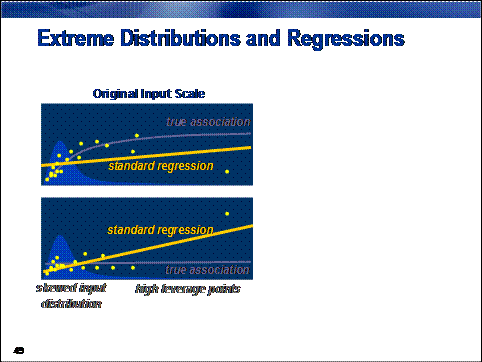
Classical regression analysis makes no assumptions about the distribution of inputs. The only assumption is that the expected value of the target (or some function thereof) is a linear combination of input measurements.

Why should you worry about extreme input distributions?

There are at least two compelling reasons.

First, in most real-world applications, the relationship between expected target value and input value does not increase without bound. Rather, it typically tapers off to some horizontal asymptote. Standard regression models are unable to accommodate such a relationship.

Second, as a point expands from the overall mean of a distribution, the point has more influence, or leverage, on model fit. Models built on inputs with extreme distributions attempt to optimize fit for the most extreme points at the cost of fit for the bulk of the data, usually near the input mean. This can result in an exaggeration or an understating of an input's association with the target, or both.

The first concern can be addressed by abandoning standard regression models for more flexible modeling methods. Abandoning standard regression models is often done at the cost of model interpretability and, more importantly, failure to address the second concern: leverage.

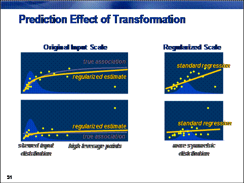
A simpler and, arguably, more effective approach is to transform offending inputs to less extreme forms and build models on these transformed inputs, which not only reduces the influence of extreme cases, but also creates an asymptotic association between input and target on the original input scale.

Transforming Inputs

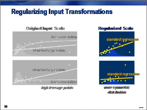
Regression models (such as clustering models) are sensitive to extreme or outlying values in the input space. Inputs with highly skewed or highly kurtotic distributions can be selected over inputs that yield better overall predictions. To avoid this problem, analysts often regularize the input distributions using a simple transformation. The benefit of this approach is improved model performance. The cost, of course, is increased difficulty in model interpretation.

The Transform Variables tool enables you to easily apply standard transformations (in addition to the specialized ones seen in Chapter 3) to a set of inputs.

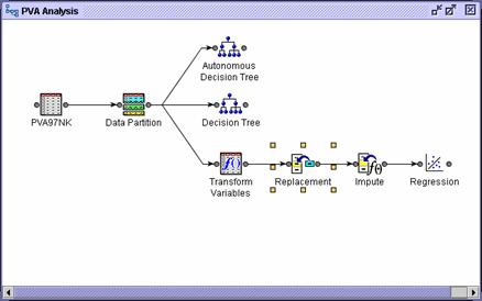
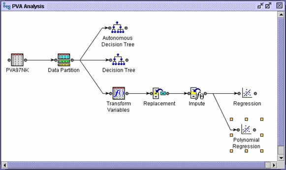
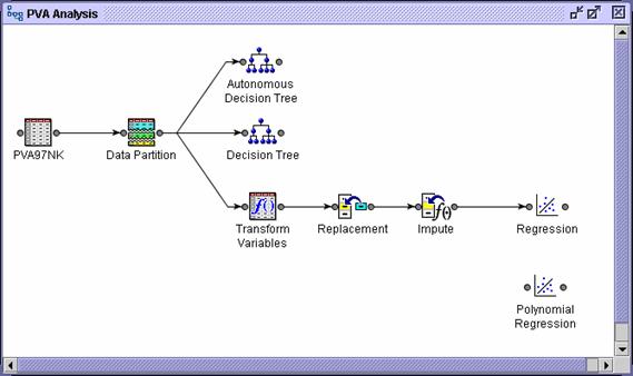
Remove the connection between the Data Partition node and the Impute node.

Select the Modify tab.

Drag a Transform Variables tool into the diagram workspace.

Connect the Data Partition node to the Transform Variables node.

Connect the Transform Variables node to the Impute node.

Adjust the diagram icons for aesthetics.

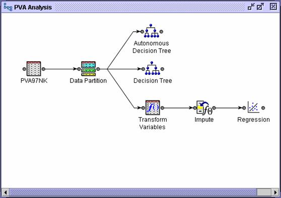
The Transform Variables node is placed before the Impute node to keep the imputed values at the average (or center of mass) of the model inputs.

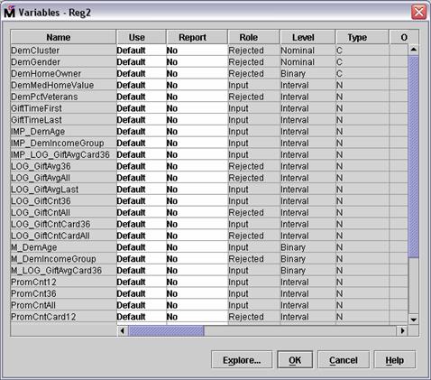
Select the Variables . property of the Transform Variables node.

The Variables - Trans window opens.

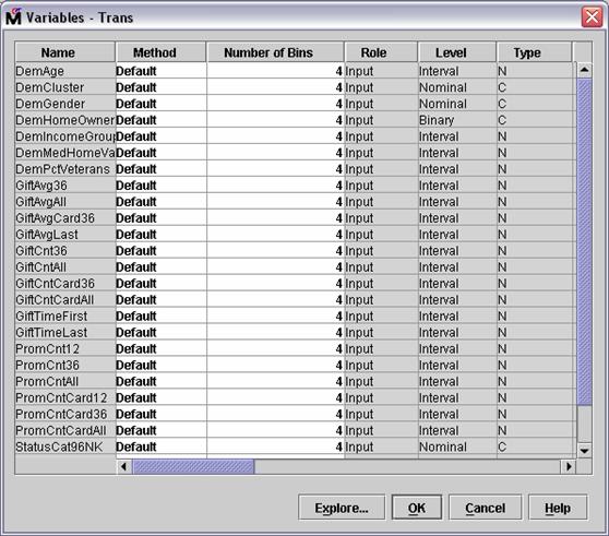
Select all inputs with Gift in the name.

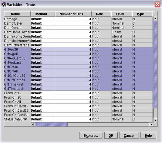
Select Explore . . The Explore window opens.

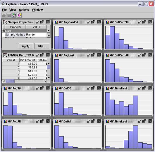
The GiftAvg and GiftCnt inputs show some degree of skewness in their distribution. The GiftTime inputs do not. To regularize the skewed distributions, use the log transformation. For these inputs, the order of magnitude of the underlying measure will predict the target rather than the measure itself.

Close the Explore window.

Deselect the two inputs with GiftTime in their names.

Select Method Log for one of the remaining selected inputs. The selected method changes from Default to Log for the GiftAvg and GiftCnt inputs.

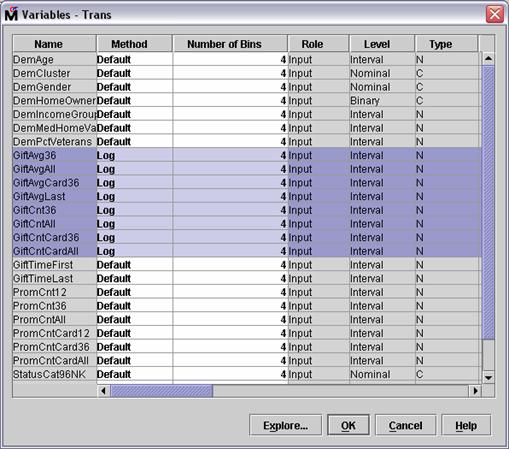
Select OK to close the Variables - Trans window.

Run the Transform Variables node and view the results.

Maximize the Output window and examine lines 20-30.

Notice the Formula column. While a log transformation was specified, the actual transformation used was log(input + 1). This default action of the Transform Variables tool avoids problems with 0-values of the underlying inputs.

Close the Transform Variables - Results window.

Run the diagram from the Regression node and view the results.

Examine lines 1653 to 1680 the Output window.

The stepwise selection process took 16 steps, and the selected model came from step 15. Notice that many of the inputs selected are log transformations of the original.

Lines 1710 to 1750 show more statistics from the selected model.

Select View Model Iteration Plot.

Again, the selected model (based on minimum average squared error) occurs in step 15. The actual value of average squared error for this model is slightly lower than that for the model with the untransformed inputs.

Select Select Chart Misclassification Rate.

The misclassification rate with the transformed input is also lower than that for the untransformed inputs. However, the model with the lowest misclassification rate comes from step 6. If you want to optimize on misclassification rate, you must change this property in the Regression node's property sheet.

Categorical Inputs

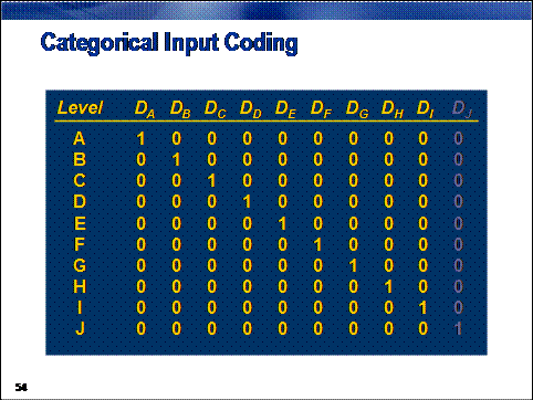
Categorical inputs present another problem for regressions. To represent these non-numeric inputs in a model, you must convert them to some sort of numeric values. This conversion is most commonly done by creating design variables (or dummy variables), with each design variable representing, roughly, one level of the categorical input. (The total number of design variables required is, in fact, one less than the number of inputs.) A single categorical input can vastly increase a model's degrees of freedom, which, in turn, increases the chances of a model overfitting.

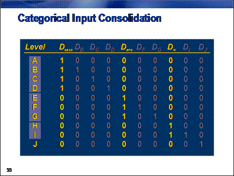
There are many remedies to this problem. One of the simplest remedies is to use domain knowledge to reduce the number of levels of the categorical input.

Recoding Categorical Inputs

The demonstration shows how to use the Replacement tool to facilitate combining input levels.

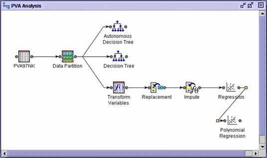
Remove the connection between the Transform Variables node and the Impute node.

Select the Modify tab.

Drag a Replacement tool into the diagram workspace.

Connect the Transform Variables node to the Replacement node.

Connect the Replacement node to the Impute node.

Select Replacement Editor . from the Replacement node Properties panel. A confirmation dialog box opens.

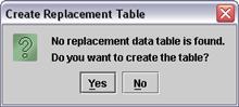
Select Yes. The Replacement Editor opens.

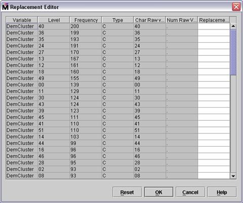
The Replacement Editor lists all levels of all categorical inputs. You can use the Replacement column to reassign values to any of the levels.

The input with the largest number of levels is DemCluster, which has so many levels that consolidating the levels using the Replacement Editor would be an arduous task. (Another, autonomous method for consolidating the levels of DemCluster (or any categorical input) is presented as a special topic in Chapter 9.)

For this demonstration, combine the levels of another input, StatusCat96NK

Scroll the Replacement Editor to view the levels of StatusCat96NK

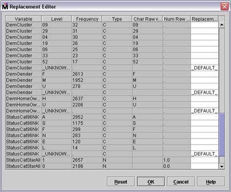
The input has six levels, plus a level to represent unknown values (which do not occur in the training data). The levels of StatusCat96NK will be consolidated as follows:

Levels A and S (active and star donors) indicate consistent donors and are grouped into a single level, A.

Levels F and N (first-time and new donors) indicate new donors and are grouped into a single level, N.

Levels E and L (inactive and lapsing donors) indicate lapsing donors and are grouped into a single level L.

Type A in the Replacement field for StatusCat96NK levels A and S.

Type N in the Replacement field for StatusCat96NK levels F and N.

Type L in the Replacement field for StatusCat96NK levels L and E.

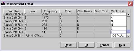
Select OK to close the Replacement Editor.

Run the Replacement node and view the results.

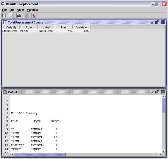
The Total Replacement Counts window shows the number of replacements that occurr in the training and validation data.

Select View Model Replaced Levels. The Replaced Levels window opens.

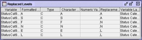
The replaced level values are consistent with expectations.

Close the Results window.

Run the Regression node and view the results.

View lines 2310-2340 of the Output window.

The REPL_StatusCat96NK input (created from the original StatusCat96NK input) is included in the stepwise selection process. The three-level input is represented by two degrees of freedom.

View lines 2422-2423 of the Output window.

Based on the odds ratios, active donors in the 96NK campaign are less likely than new donors to contribute in the 97NK campaign. On the other hand, lapsing donors in the 96NK campaign are more likely than new donors to contribute in the 97NK campaign.

Select View Model Iteration Plot.

The selected model from step 19 has, again, a slightly smaller average squared error than previous models.

Polynomial Regressions

The Regression tool assumes (by default) a linear and additive association between the inputs and the logit of the target. If the true association is more complicated, such an assumption might result in biased predictions. For decisions and rankings, this bias can (in some cases) be unimportant. For estimates, this bias will appear as a higher value for the validation average squared error fit statistic.

In the dot color problem, the (standard logistic regression) assumption that the concentration of yellow dots increases toward the upper-right corner of the unit square seems to be suspect.

When minimizing prediction bias is important, you can increase the flexibility of a regression model by adding polynomial combinations of the model inputs. This enables predictions to better match the true input/target association. It also increases the chances of overfitting while simultaneously reducing the interpretability of the predictions. Therefore, polynomial regression must be approached with some care.

In SAS Enterprise Miner, adding polynomial terms can be done selectively or autonomously.

Adding Polynomial Regression Terms Selectively

This demonstration shows how to selectively add polynomial regression terms.

You can modify the existing Regression node or add a new Regression node. If you add a new node, you must configure the Polynomial Regression node to perform the same tasks as the original. An alternative is to make a copy of the existing node.

Right-click the Regression node and select Copy from the menu.

Right-click the diagram workspace and select Paste from the menu. A new Regression node is added with the label Regression (2) to distinguish it from the existing one.

Select the Regression (2) node. The properties are identical to the existing node.

Rename the new regression node Polynomial Regression

Connect the Polynomial Regression node to the Impute node.

The Term Editor enables you to add specific polynomial terms to the regression model.

Select Term Editor . from the Polynomial Regression Properties panel. The Terms dialog box opens.

Suppose that you suspect an interaction between home value and time since last gift. (Perhaps a recent change in property values affected the donation patterns.)

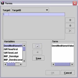
Select DemMedHomeValue in the Variables panel of the Terms dialog box.

Select the Add button, . The DemMedHomeValue input is added to the Term panel.

Repeat for GiftTimeLast

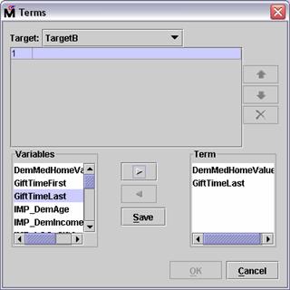
Select Save. An interaction between the selected inputs is now available for consideration by the regression node.

Similarly, suppose that you suspect a parabola-shaped relationship between donation and donor age. (Donation odds increase with age, peak, and then decline with age.)

Select IMP_DemAge

Select the Add button, . The IMP_DemAge input is added to the Term panel.

Select the Add button, again. Another IMP_DemAge input is added to the Term panel.

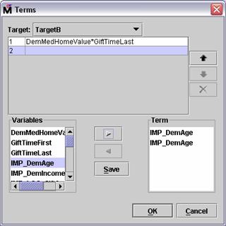
Select Save. A quadratic age term is available for consideration by the model.

Select OK to close the Terms dialog box.

To use the terms you defined in the Terms dialog box, you must enable the User Terms option in the Regression node.

Select User Terms Yes in the Polynomial Regression Properties panel.

Run the Polynomial Regression node and view the results.

Scroll the Output window to lines 2515-2540.

The stepwise selection summary shows the polynomial terms added in steps 3 and 8.

View the Iteration Plot window.

While present in the selected model, the interaction terms appear to have negligible effect on the model performance (at least for average squared error).

This begs the question: How do you know which non-linear terms to include in a model?

Unfortunately, there is no simple solution to this question in SAS Enterprise Miner, short of trying all of them

Adding Polynomial Regression Terms Autonomously
(Self-Study)

SAS Enterprise Miner has the ability to add every polynomial combination of inputs to a regression model. Obviously, this feature must be used with some care, because the number of polynomial input combinations increases rapidly with input count.

For instance, the PVA97NK data set has 20 interval inputs. If you want to consider every quadratic combination of these 20 inputs, your selection procedure must sequentially slog through more than 200 inputs. This is not an overwhelming task for today's fast computers, but there is a shortcut that many analysts use to reduce this count.

The trick is to only consider polynomial expressions of those inputs found to be linearly related to the logit of the target. That is, start with those inputs selected by the original regression model. A simple modification to your analysis diagram makes this possible.

Delete the connection between the Impute node and the Polynomial Regression node.

Connect the Regression node to the Polynomial Regression node.

Right-click the Polynomial Regression node and select Update from the menu. A Status dialog box informs you of the completion of the update process.

Select OK to close the Status dialog box.

Select Variables . from the Polynomial Regression Properties panel.

All inputs not selected in the original regression's stepwise procedure are rejected.

Select OK to close the Variables dialog box.

Select Polynomial Terms Yes in the Polynomial Regression Properties panel. This adds all quadratic combinations of the interval inputs.

You can increase this to a higher order polynomial by changing the Polynomial Degree field.

Select User Terms No. The terms added in the last demonstration will be included by specifying the Polynomial Terms option.

Run the Polynomial Regression node and view the results. (This might take a few minutes to complete on slower computers.)

Scroll to the bottom of the Output window.

The amount of output generated by the selection history exceeds the 10,000-line, client-transfer limit of SAS Enterprise Miner. To view the complete output listing, you must open the referenced file.

Doing so reveals a 121-step and 18,000-line input selection free-for-all. The selection summary is shown below.

(Continued on the next page.)

(Continued on the next page.)

Examine the iteration plot.

Surprisingly, the selected model comes from step 12 and involves only a few regression terms.

Unfortunately, all but one of the selected terms is an interaction.

While this model is the best predictor of PVA97NK response found up to this time, it is nearly impossible to interpret. This is an important factor to remember when considering polynomial regression models.

Exercises

Predictive Modeling Using Regression

Return to the Chapter 4 Organics diagram in the Exercises project. Explore the ORGANICS data source.

In preparation for regression, is any missing values imputation needed? If yes, should you do this imputation before generating the decision tree models? Why or why not?

Add an Impute node to the diagram and connect it to the Data Partition node.

Change Default Input Method to Tree for both class and interval variables. Create missing value indicator variables. Replace missing values for GENDER with U for unknown.

Add a Regression node to the diagram and connect it to the Impute node.

Choose the stepwise selection and average squared error as the selection criterion.

Run the Regression node and view the results. Which variables are included in the final model? Which variables are important in this model?

In preparation for regression, are any transformations of the data warranted? Why or why not?

Add a Transform Variables node to the diagram and connect it to the Impute node.

The variable AFFL appears to be skewed to the right. Use a square root transformation for AFFL. The variables BILL and LTIME also appear to be skewed to the right. Use SAS Enterprise Miner to transform these variables to maximize normality.

Run the Transform Variables node. Explore the exported training data. Did the transformation of AFFL appear to result in a less skewed distribution? What transformation was chosen for the variables BILL and LTIME

Add another Regression node to the diagram and connect it to the Transform Variables node.

Choose the stepwise selection method and average squared error selection criterion.

Run this new Regression node and view the results. Which variables are included in the final model? Which variables are important in the model?

How do the validation average squared errors of the two regression models compare? How do the regression models compare to the tree models?

Chapter Summary

Regression models are a prolific and useful way to create predictions. New cases are scored using a prediction formula. Inputs are selected via a sequential selection process. Model complexity is controlled by fit statistics calculated on validation data.

To use regression models, there are several issues with which to contend that go beyond the predictive modeling essentials. First, a mechanism for handling missing input values must be included in the model development process. Second, methods for handling extreme or outlying predictions should be included. Third, the level-count of a categorical should be reduced to avoid overfitting. Finally, the model complexity might need to be increased beyond what is provided by standard regression methods. One approach to this is polynomial regression. Polynomial regression models can be fit by hand with specific interactions in mind. They also can be fit autonomously by selecting polynomial terms from a list of all polynomial candidates.

Solutions to Exercises

Predictive Modeling Using Regression

Right-click the ORGANICS data source in the Project Panel and select Explore.

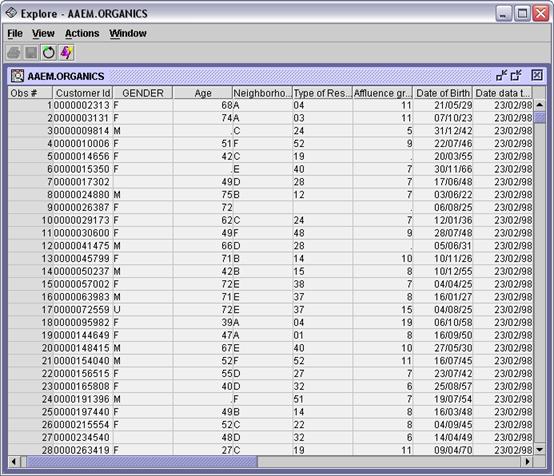
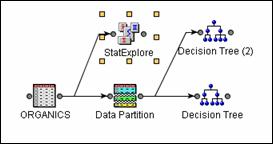
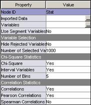
Examine the ORGANICS data table to reveal several inputs with missing values. A more precise way to determine the extent of missing values in this data set is to use the StatExplore node.

Connect a StatExplore node to the ORGANICS data source in the diagram workspace.

Select the StatExplore node in the diagram and examine the Properties panel.

Change the option to Hide Rejected Variables to No and change the option for Interval Variables to Yes using the menus.

Run the StatExplore node and examine the Output window in the Results.

The variable GENDER has a relatively large number of missing values.

The variables AFFL and AGE have over 1000 missing values each.

Imputation of missing values should be done prior to generating a regression model. However, imputation is not necessary before generating a decision tree model because a decision tree can use missing values in the same way as any other data value in the data set.

Close the StatExplore node results and return to the diagram workspace.

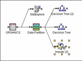
After you add an Impute node, the diagram should appear as shown below.

Choose the imputation methods.

Select the Impute node in the diagram.

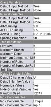
To use tree imputation as the default method of imputation, change the Default Input Method for both class and interval variables to Tree using the menus.

To create missing value indicator variables, change the Indicator Variable property to Unique and the Indicator Variable Role to Input using the menus in the Properties panel.

To replace missing values for the variable GENDER with U, first change Default Character Value to U. The Properties panel should appear as shown.

Select Variables . . Change the value in the Method column for the variable GENDER to Constant as shown below.

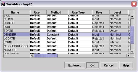
Select OK to confirm the change.

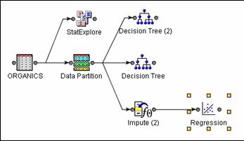
Add a Regression node to the diagram as shown below.

Choose the stepwise selection and average squared error as the selection criterion.

Select the Regression node in the diagram.

Select Selection Model Stepwise.

Select Selection Criterion Validation Error.

Run the Regression node and view the results. The Output window shows which variables are in the final model and which variables are important.

Line 658 lists the inputs included in the final model:

Important inputs can be ascertained by Wald Chi-Square, standardized estimates, and odds ratio estimates.

Important inputs include IMP_AFFL IMP_AGE, and IMP_GENDER

Close the regression results and return to the diagram workspace.

Explore the input distributions.

Select the ORGANICS node and select Variables . in the Properties panel.

Select all interval input variables.

Select Explore . .

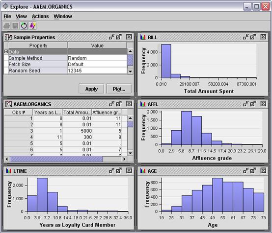
The variables AFFL BILL, and LTIME are skewed to the right and might need to be transformed for a regression. This is evident in the histograms that can be viewed in the exploration tool available in the Input Data node and other nodes.

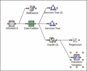
Connect a Transform Variables node as shown below.

Transform inputs.

Select Variables . in the Transform Variables node's Properties panel.

In the Method column for the variable IMP_AFFL, select Square Root from the menu. In the Method column for the variables BILL and IMP_LTIME, select Max. Normal from the menu. The Variables window should appear as shown below.

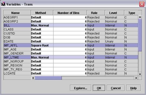
Select OK to confirm the changes.

Run the Transform Variables node. Do not view the results. Instead, select Exported Data . from the Transform Variables node's Properties panel. The Exported Data - Transform Variables window opens.

Select the Train data set and select Explore . .

In the Explore window, select Actions Plot . .

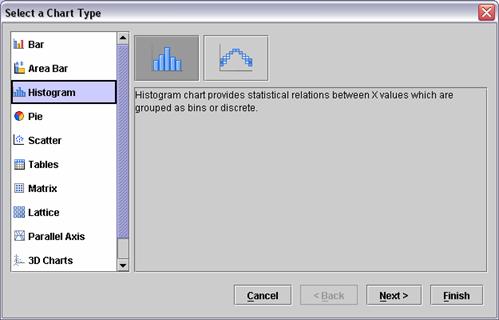
Select Histogram as the type of chart and then select Next >.

Change the role of SQRT_IMP_AFFL to X.

Select Finish.

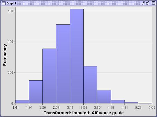
The transformed variable appears to be less skewed than the original variable.

To view the transformations for the other variables, close the graph and examine the Transformations window in the results. The transformation chosen for the variable BILL was a square root transformation, and the transformation for IMP_LTIME was the fourth root. You can confirm this by opening the Results window and viewing lines 28-25 of the output.

Close the results and return to the diagram workspace.

Add a second Regression node to the diagram as shown below.

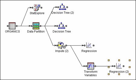
Choose the stepwise selection and average squared error as the selection criterion.

Select the Regression node in the diagram.

Select Selection Model Stepwise.

Select Selection Criterion Validation Error.

Run the Regression node and view the results. The Output window shows which variables are in the final model and which variables are important.

Line 563 lists the inputs included in the final model:

Important inputs can be ascertained by Wald Chi-Square, standardized estimates, and odds ratio estimates.

Important inputs include SQRT_IMP_AFFL IMP_AGE, and IMP_GENDER

Model fit comparisons.

Examine the Fit Statistics window.

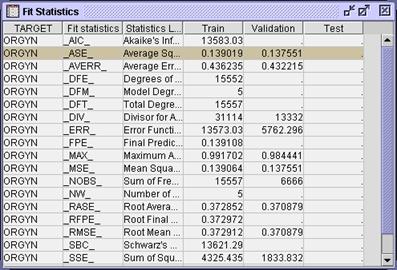
The validation average squared error for this model equals 0.1376.

Open the Results window for the original regression and examine the Fit Statistics window.

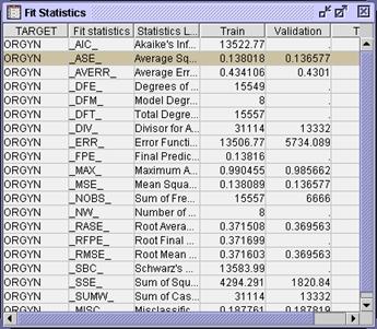
The validation average squared error for the original regression model equals 0.1365, or slightly lower. In this case, transforming the inputs does not improve model fit.

Open the Results window for the original tree model and examine the Fit Statistics window.

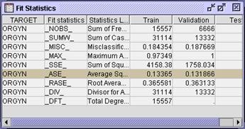
The average squared error of the tree model is smaller. It appears that the regression models are less adept at modeling the association between inputs and target.