Matematica si Informatica in limba
Engleza
Traffic shaping. QoS application
Chapter 1
1.1 Introduction
The
past three centuries have been dominated by the progress of technology. The
18th century was the era of the great mechanical systems and the Industrial
Revolution. The 19th century was the age of the steam engine. During the 20th
century, the technology was gathering information, processing, and distribution
of it. Among other developments, we saw the birth and unprecedented growth of
the computer industry.
The history of computer networking is complex, involving
many people from all over the world over the past thirty years. In the 1940s,
computers were huge electromechanical devices that were prone to failure. In
1947, the invention of a semiconductor transistor opened up many possibilities
for making smaller, more reliable computers. In the 1950s, mainframe computers,
run by punched card programs, began to be commonly used by large institutions.
In the late 1950s, the integrated circuit - that combined several, many, and
now millions, of transistors on one small piece of semiconductor - was
invented. Through the 1960s, mainframes with terminals were common place, and
integrated circuits became more widely used.
In the
late 60s and 70s, smaller computers, called minicomputers (though still huge by
today's standards), came into existence. In 1978, the Apple Computer company
introduced the personal computer. In 1981, IBM introduced the open-architecture
personal computer. The user friendly Mac, the open architecture IBM PC, and the
further micro-miniaturization of integrated circuits lead to widespread use of
personal computers in homes and businesses. As the late 1980s began, computer
users - with their stand-alone computers - started to share data (files) and
resources (printers). People asked, why not connect them?
Starting
in the 1960s and continuing through the 70s, 80s, and 90s, the Department of
Defense (DoD) developed large, reliable, wide area networks (WANS). Some of
their technology was used in the development of LANs, but more importantly, the
DoDs WAN eventually became the Internet.
Somewhere
in the world, there were two computers that wanted to communicate with each
other. In order to do so, they both needed some kind of device that could talk
to the computers and the media (the Network Interface Card - NIC), and
some way for the messages to travel (medium).
Suppose, also, that the
computers wanted to communicate with other computers that were a great distance
away. The answer to this problem came in the form of repeaters and hubs. The
repeater (an old device used by telephone networks) was introduced to enable
computer data signals to travel farther. The multi-port repeater, or hub,
was introduced to enable a group of users to share files, servers and
peripherals. You might call this a workgroup
network.
Soon, work groups
wanted to communicate with other work groups. Because of the functions of hubs
(they broadcast all messages to all ports, regardless of destination), as the
number of hosts and the number of workgroups grew, there were larger and larger
traffic jams. The bridge was
invented to segment the network, to introduce some traffic control.
The
best feature of the hub - concentration /connectivity - and the best feature of
the bridge - segmentation - were combined to produce a switch. It had lots of ports, but allowed each port to pretend it
had a connection to the other side of the bridge, thus allowing many users and
lots of communications.
In the
mid-1980s, special-purpose computers, called gateways (and then routers)
were developed. These devices allowed the interconnection of separate LANs. Internetworks were created. The DoD
already had an extensive internetwork, but the commercial availability of
routers - which carried out best path
selections and switching for data
from many protocols - caused the explosive growth of networks .
As the chart shows,
the Web has experienced three growth stages:
- 1991-1997: Explosive growth, at a rate of 850%
per year.
- 1998-2001: Rapid growth, at a rate of 150%
per year.
- 2002-2006: Maturing growth, at a rate of 25%
per year.
The
number of Internet websites each year since the Web's
founding.
Today
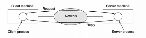
many companies have a substantial number of computers . For example an ISP can
have multiple computers in different locations. The main computer can be
situated in one region and the others in the neighbourhood. Making the data
available to anyone on the network without regard to the physical location of
the resource and the user is called resource sharing. The data is stored on
powerfull computer called server. The
employees have simpler machines, called clients, with which they access
remote data.
Broadly
speaking, there are two types of transmission technology that are in widespread
use. They are as follows:
Broadcast links.
Point-to-point links.
Broadcast
networks have a single communication channel
that is shared by all the machines on the network. Short messages, called packets
in certain contexts, sent by any machine are received by all the others. An
address field within the packet specifies the intended recipient. Upon
receiving a packet, a machine checks the address field. If the packet is intended
for the receiving machine, that machine processes the packet; if the packet is
intended for some other machine, it is just ignored.
Broadcast
systems generally also allow the possibility of addressing a packet to all destinations by using a special code in the
address field. When a packet with this code is transmitted, it is received and
processed by every machine on the network in the same time. This mode of
operation is called broadcasting. Some broadcast systems also support
transmission to a subset of the machines, and this is known as multicasting.
When a packet is sent to a certain group, it is delivered to all machines
subscribing to that group.
Point-to-point networks consist of many connections between individual pairs of
machines. To go from the source to the destination, a packet on this type of
network may have to first visit one or more intermediate machines. Often
multiple routes, of different lengths, are possible, so finding good ones is
important in point-to-point networks. Point-to-point transmission with one
sender and one receiver is called unicasting.
1.2 Classification of networks
A
criteria for classifying networks is their scale. At the top are the personal area
networks, networks that are meant for one person. For example, a wireless
network connecting a computer with its mouse, keyboard, and printer is a
personal area network. Beyond the personal area networks come longer-range
networks. These can be divided into local, metropolitan, and wide area
networks. Finally, the connection of two or more networks is called an
internetwork. The worldwide Internet is a well-known example of an internetwork

1.2.1 Local Area Networks
Local
area networks, generally called LANs,
are networks within a single building or campus of up to a few kilometers in
size. They are widely used to connect personal computers and workstations in
offices or at home to share resources (e.g., printers) and exchange
information. LANs are distinguished from other kinds of networks by three
characteristics:
(1) their size,
(2) their transmission
technology ,
(3) their topology.
LANs may
use a transmission technology consisting of a cable to which all the machines
are attached. Traditional LANs run at speeds of 10 Mbps to 100 Mbps, have low
delay (microseconds or nanoseconds), and make very few errors.
LANs may
have various topologies . By
topology we undestant the structure of the network. The
topolgy can be devided in two parts, the physical topology, which is the actual
layout of the wire (media), and the logical topology, which defines how the
media is accessed by the hosts. The physical topologies that are commonly used
are the Bus, Ring and Star.
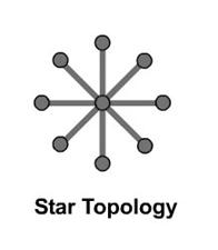
In a star topology, each network device has
a lot of cable which connects to the central node , giving each device a
separate connection to the network. If there is a problem with a cable, it will
generally not affect the rest of the network. The most common cable media in
use for star topologies is unshielded twisted pair copper cabling. Category 3
is still found frequently in older installations. It is capable of 10 megabits
per second data transfer rate, making it suitable for only 10 BASE T Ethernet. Most new installations use Category 5 cabling.
It is capable of data transfer rates of 100 megabits per second, enabling it to
employ 100 BASE T Ethernet, also
known as Fast Ethernet. More
importantly, the brand new 1000 BASE T Ethernet standard will be able to run
over most existing Category 5. Finally, fiber optic cable can be used to
transmit either 10 BASE T or 100 BASE T Ethernet frames.
When using Category 3 or 5 twisted pair cabling,
individual cables cannot exceed 100 meters.
Advantages
- More suited for larger networks
- Easy to expand network
- Easy to troubleshoot because problem usually
isolates itself
- Cabling types can be mixed
Disadvantages
- Hubs become a
single point of network failure, not the cabling
- Cabling more
expensive due to home run needed for every device
Best used in small area
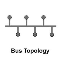
of network. In the bus topology the
cable runs from computer to computer making each computer a link of a chain.
Different types of cable determine
way of network can be connected.
Advantages of a Linear Bus Topology
- Easy to connect a computer or peripheral to a
linear bus.
- Requires less cable length than a star topology.
Disadvantages of a Linear Bus Topology
- Entire network shuts down if there is a break in
the main cable.
- Terminators are required at both ends of the
backbone cable.
- Difficult to identify the problem if the entire
network shuts down.
- Not meant to be used as a stand-alone solution in
a large building.
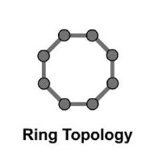
Ring topologies are used on token ring networks. Each device processes
and retransmits the signal, so it is capable of supporting many devices in a
somewhat slow but very orderly fashion. A token, or small data packet, is
continuously passed around the network. When a device needs to transmit, it
reserves the token for the next trip around, then attaches its data packet to
it. The receiving device sends back the packet with an acknowledgment of
receipt, then the sending device puts the token back out on the network. Most
token ring networks have the physical cabling of a star topology and the
logical function of a ring through use of multi
access units (MAU). In a ring topology, the network signal is passed
through each network card of each device and passed on to the next device. All
devices have a cable home runned back to the MAU. The MAU makes a logical ring
connection between the devices internally. When each device signs on or off, it
sends an electrical signal which trips mechanical switches inside the MAU to
either connect the device to the ring or drop it off the ring. The most common
type of cabling used for token ring networks is twisted pair. Transmission
rates are at either 4 or 16 megabits per second.
Advantages
- Very orderly network where every device has access
to the token and the opportunity to transmit
- Performs better than a star topology under heavy
network load
- Can create much larger network using Token Ring
Disadvantages
- One malfunctioning workstation or bad port in the
MAU can create problems for the entire network
- Moves, adds and changes of devices can affect the
network
- Network adapter cards and MAU's are much more
expensive than Ethernet cards and hubs
- Much slower than
an Ethernet network under normal load
1.2.2 Metropolitan Area Networks
Metropolitan Area Networks called MAN are optimized
for a larger geographical area than is a LAN, ranging from several blocks of
buildings to entire cities. As with local networks, MANs can also depend on
communications channels of moderate-to-high data rates. They typically use
wireless infrastructure or optical fiber connections for linking.
A
MAN might be owned and operated by a single organization, but it usually will
be used by many individuals and organizations. MANs might also be owned and
operated as public utilities. They will often provide means for internetworking
of local networks.
1.2.3 Wide Area Networks
A wide area network, or WAN, spans a large geographical area, often a
country or continent. It contains a collection of machines intended for running
user (i.e., application) programs. We will follow traditional usage and call
these machines hosts.
The hosts are connected by a communication
subnet, or just subnet for
short. The job of the subnet is to carry messages from host to host.
In this model each host is frequently connected to a LAN
on which a router is present, although in some cases a host can be connected
directly to a router. The collection of communication lines and routers (but
not the hosts) form the subnet.
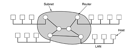
Relation between hosts on LANs
and the subnet.
In most
WANs, the network contains numerous transmission lines, each one connecting a
pair of routers. If two routers that do not share a transmission line wish to
communicate, they must do this indirectly, via other routers. When a packet is
sent from one router to another via one or more intermediate routers, the
packet is received at each intermediate router in its entirety, stored there until
the required output line is free, and then forwarded. A subnet organized
according to this principle is called a store-and-forward or packet-switched
subnet. Nearly all wide area networks (except those using satellites) have
store-and-forward subnets. When the packets are small and all the same size,
they are often called cells.
The
principle of a packet-switched WAN is so important that it is worth devoting a
few more words to it. Generally, when a process on some host has a message to
be sent to a process on some other host, the sending host first cuts the
message into packets, each one bearing its number in the sequence. These
packets are then injected into the network one at a time in quick succession.
The packets are transported individually over the network and deposited at the
receiving host, where they are reassembled into the original message and
delivered to the receiving process. A stream of packets resulting from some
initial message is illustrated below:
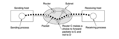
In the figure above, all the packets follow the route ACE, rather
than ABDE
or ACDE.
In some networks all packets from a given message must
follow the same route; in others each packet is routed separately. Of course,
if ACE
is the best route, all packets may be sent along it, even if each packet is
individually routed.
Routing decisions are made locally. When a packet arrives at router A,itis up to A to
decide if this packet should be sent on the line to B
or the line to C. How A
makes that decision is called the routing algorithm.
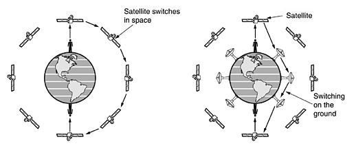
Not all WANs are packet switched. A second possibility for a WAN is a
satellite system. Each router has an antenna through which it can send and
receive. All routers can hear the output from
the satellite, and in some cases they can also hear the upward transmissions of
their fellow routers to the satellite as well.
Sometimes the routers are connected to a substantial point-to-point subnet,
with only some of them having a satellite antenna.
1.2.4. Wireless networks
Digital wireless communication is not a new idea. As early as 1901, the
Italian physicist Guglielmo Marconi demonstrated a ship-to-shore wireless
telegraph, using Morse Code (dots and dashes are binary, after all). Modern
digital wireless systems have better performance, but the basic idea is the
same.
Wireless networks can be divided into three main categories:
System interconnection.
Wireless LANs. (WLAN)
Wireless WANs. (WWAN)
System interconnection is all about interconnecting the components of a compute using
short-range radio. Almost every computer has a monitor, keyboard, mouse, and
printer connected to the main unit by cables. Some companies got together to
design a short-range wireless network called Bluetooth
to connect these components without wires. Bluetooth
also allows digital cameras, headsets, scanners, and other devices to connect
to a computer by merely being brought within range. No cables, no driver
installation, just put them down, turn them on, and they work. Many people,
prefer this facility.
In the simplest form, system interconnection networks use the
master-slave paradigm (see the figure below). The system unit is normally the
master, talking to the mouse, keyboard, etc., as slaves. The master tells the
slaves what addresses to use, when they can broadcast, how long they can transmit,
what frequencies they can use, and so on.
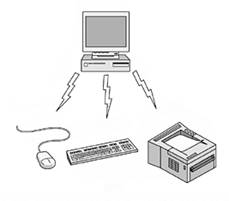
Bluetooth/Wireless
connection
Wireless LANs are systems in which every computer has a radio modem and antenna with
which it can communicate with other systems. Often there is an antenna on the
ceiling that the machines talk to. If the systems are close enough, they can
communicate directly with one another in a peer-to-peer configuration.
Wireless LANs are becoming increasingly common in small offices and
homes, where we don't want to install
Ethernet and get rid of the cables.
Wirless LAN
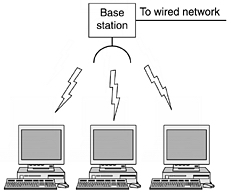
Wide Area Systems . The radio
network used for cellular telephones is an example of a low-bandwidth wireless
system. Cellular wireless networks are like wireless LANs, except that the
distances involved are much greater and the bit rates much lower. Wireless LANs
can operate at rates up to about 50 Mbps over distances of tens of meters.
Cellular systems operate below 1 Mbps, but the distance between the base
station and the computer or telephone is measured in kilometers rather than in
meters.
Example of wide area systems
Home Networks
Home networking is on the horizon. The fundamental idea
is that in the future most homes will be set up for networking. Every device in
the home will be capable of communicating with every other device, and all of
them will be accessible over the Internet. This is one of those visionary
concepts that nobody asked for (like TV remote controls or mobile phones), but
once they arrived nobody can imagine how they lived without them.
Many devices are capable of being networked. Some of the
more obvious categories (with examples) are as follows:
Computers (desktop PC, notebook PC, PDA, shared peripherals).
Entertainment (TV, DVD, VCR, camcorder, camera, stereo, MP3).
Telecommunications (telephone, mobile telephone, intercom, fax).
Appliances (microwave, refrigerator, clock, aircooler, lights).
Home computer networking is already here in a limited way. Many homes
already have a device to connect multiple computers to a fast Internet
connection. Networked entertainment is not quite here, but as more and more
music and movies can be downloaded from the Internet, there will be a demand to
connect stereos and televisions to it. Also, people will want to share their
own videos with friends and family, so the connection will need to go both
ways. Telecommunications gear is already connected to the outside world, but
soon it will be digital and go over the Internet. Finally, remote monitoring of
the home and its contents is a likely winner. Probably many parents would be
willing to spend some money to monitor their sleeping babies on their PDAs when
they are eating out.
Home networking has some fundamentally different properties than other
network types. First, the network and devices have to be easy to install. The
author has installed numerous pieces of hardware and software on various
computers over the years, with mixed results. A series of phone calls to the
vendor's helpdesk typically resulted in answers like (1) Read the manual, (2)
Reboot the computer, (3) Remove all hardware and software except ours and try
again, (4) Download the newest driver from our Web site, and if all else fails,
(5) Reformat the hard disk and then reinstall Windows from the CD-ROM. Telling
the purchaser of an Internet refrigerator to download and install a new version
of the refrigerator's operating system is not going to lead to happy customers.
1.2.6 Internetworks
Many networks exist in the world, often with different hardware and software.
People connected to one network often want to communicate with people attached
to a different one. The fulfillment of this desire requires that different, and
frequently incompatible networks, be connected, sometimes by means of machines
called gateways to make the connection and
provide the necessary translation, both in terms of hardware and software. A
collection of interconnected networks is called an internetwork or internet. A
common form of internet is a collection of LANs connected by a WAN.
An internetwork is formed when distinct networks are interconnected.
1.3 OSI Reference model
To reduce their design complexity, most networks are organized as a
stack of layers.
Layer n on one machine carries on a
conversation with layer n on another machine. The rules and conventions used in this
conversation are collectively known as the layer n
protocol. Basically, a protocol is an agreement between the communicating
parties on how communication is to proceed.
A set of layers and protocols is called
a network architecture.
For this we will explain the OSI
reference model which is based on on a proposal developed by the
International Standards Organization (ISO) . The model is called the ISO OSI (Open Systems Interconnection) Reference Model
because it deals with connecting open systems-that is, systems that are open
for communication with other systems . The OSI model has seven layers.
The OSI Reference Model
Physical Layer
The physical layer, the lowest
layer of the OSI model, is concerned with the transmission and reception of the
unstructured raw bit stream over a physical medium. It describes the
electrical/optical, mechanical, and functional interfaces to the physical
medium, and carries the signals for all of the higher layers. It provides:
Data encoding: modifies the simple digital signal
pattern (1s and 0s) used by the PC to better accommodate the characteristics of
the physical medium, and to aid in bit and frame synchronization. It determines:
What
signal state represents a binary 1
How
the receiving station knows when a "bit-time" starts
How
the receiving station delimits a frame
Physical medium attachment, accommodating various
possibilities in the medium:
Transmission technique: determines whether the
encoded bits will be transmitted by baseband (digital) or broadband (analog)
signaling.
Physical medium transmission: transmits bits as
electrical or optical signals appropriate for the physical medium, and
determines:
What
physical medium options can be used
How
many volts/db should be used to represent a given signal state, using a given
physical medium
Data Link Layer
The
data link layer provides error-free transfer of data frames from one node to
another over the physical layer, allowing layers above it to assume virtually
error-free transmission over the link. To do this, the data link layer
provides:
Link
establishment and termination: establishes and terminates the logical link
between two nodes.
Frame
traffic control: tells the transmitting node to "back-off" when no frame
buffers are available.
Frame
sequencing: transmits/receives frames sequentially.
Frame
acknowledgment: provides/expects frame acknowledgments.
Detects and recovers from errors that occur in the
physical layer by retransmitting non-acknowledged frames and handling duplicate
frame receipt.
Frame
delimiting: creates and recognizes frame boundaries.
Frame
error checking: checks received frames for integrity.
Media
access management: determines when the node "has the right" to use the physical
medium.
Network Layer
The
network layer controls the operation of the subnet, deciding which physical
path the data should take based on network conditions, priority of service, and
other factors. It provides:
Routing:
routes frames among networks.
Subnet
traffic control: routers (network layer intermediate systems) can instruct a
sending station to "throttle back" its frame transmission when the router's
buffer fills up.
Frame
fragmentation: if it determines that a downstream router's maximum transmission
unit (MTU) size is less than the frame size, a router can fragment a frame for
transmission and re-assembly at the destination station.
Logical-physical
address mapping: translates logical addresses, or names, into physical addresses.
Subnet
usage accounting: has accounting functions to keep track of frames forwarded by
subnet intermediate systems, to produce billing information.
Transport Layer
The
transport layer ensures that messages are delivered error-free, in sequence, and
with no losses or duplications. It relieves the higher layer protocols from any
concern with the transfer of data between them and their peers.
The size and complexity of a transport protocol depends on the type of
service it can get from the network layer. For a reliable network layer with
virtual circuit capability, a minimal transport layer is required. If the
network layer is unreliable and/or only supports datagrams, the transport
protocol should include extensive error detection and recovery.
The transport
layer provides:
Message
segmentation: accepts a message from the (session) layer above it, splits the
message into smaller units (if not already small enough), and passes the
smaller units down to the network layer. The transport layer at the destination
station reassembles the message.
Message acknowledgment: provides reliable
end-to-end message delivery with acknowledgments.
Message traffic control: tells the transmitting
station to "back-off" when no message buffers are available.
Session multiplexing: multiplexes several message
streams, or sessions onto one logical link and keeps track of which messages
belong to which sessions (see session layer).
Typically, the transport layer can accept relatively large messages, but
there are strict message size limits imposed by the network (or lower) layer.
Consequently, the transport layer must break up the messages into smaller
units, or frames, pretending a header to each frame.
The transport
layer header information must then include control information, such as message
start and message end flags, to enable the transport layer on the other end to
recognize message boundaries. In
addition, if the lower layers do not maintain sequence, the transport header
must contain sequence information to enable the transport layer on the
receiving end to get the pieces back together in the right order before handing
the received message up to the layer above.
Session Layer
The
session layer allows session establishment between processes running on
different stations. It provides:
Session
establishment, maintenance and termination: allows two application processes on
different machines to establish, use and terminate a connection, called a
session.
Session
support: performs the functions that allow these processes to communicate over
the network, performing security, name recognition, logging, and so on.
Presentation Layer
The
presentation layer formats the data to be presented to the application layer.
It can be viewed as the translator for the network. This layer may translate data from a format
used by the application layer into a common format at the sending station, and
then translate the common format to a format known to the application layer at
the receiving station.
The presentation layer
provides:
Character
code translation: for example, ASCII to EBCDIC. (Extended Binary
Coded Decimal Interchange Code
Data
conversion: bit order, integer-floating point.
Data
compression: reduces the number of bits that need to be transmitted on the
network.
Data
encryption: encrypt data for security purposes. For example, password
encryption.
Application Layer
The
application layer serves as the window for users and application processes to
access network services. This layer contains a variety of commonly needed functions:
Resource
sharing and device redirection
Remote
file access
Remote
printer access
Inter-process
communication
Network
management
Directory
services
Electronic
messaging (such as mail)
Network
virtual terminals
By creating specifications on multiple layers, the OSI model has a
lot of benefits:
Reduced complexity allows faster evolution. There are companies
specialized in creating products specific for one layer, instead of rebuilding
everything from the application to the physical layer.
Interoperability is much easier due to standardization.
Each layer uses the service of the layer immediately below it, and
so it is easier to remember what the lower layer does.
It simplifies teaching. For example, network administrators need
to know the functions of the lowest four layers, while programmers need to know
the upper layers.
Units and metrics
To avoid any confusion metric units are used instead of traditional
units. The principal metric prefixes are listed in the figure below. The
prefixes are typically abbreviated by their first letters, with the units
greater than 1 capitalized (KB, MB, etc.). One exception (for historical
reasons) is kbps for kilobits/sec. Thus, a 1-Mbps communication line transmits
106 bits/sec and a 100 psec (or 100 ps) clock ticks every 10-10
seconds. Since milli and micro both begin with the letter ''m,'' a choice had
to be made. Normally, ''m'' is for milli and ''µ'' (the Greek letter mu) is for
micro.
|
Exp
|
Explicit
|
Prefix
|
Exp
|
Explicit
|
Prefix
|
|
|
mili
|
|
|
Kilo
|
|
|
micro
|
|
|
Mega
|
|
|
nano
|
|
|
Giga
|
|
|
pico
|
|
|
Tera
|
|
|
femto
|
|
|
Peta
|
|
|
atto
|
|
|
Exa
|
|
|
zepto
|
|
|
Zetta
|
|
|
yocto
|
|
|
Yotta
|
Here
kilo means 210 (1024) rather than 103 (1000) because memories are always a power of two .
Thus:
1-KB memory contains 210(1024) bytes, not
1000 bytes.
1-MB memory contains 220 (1,048,576) bytes
1-GB memory contains 230 (1,073,741,824) bytes
1-TB database contains 240 (1,099,511,627,776)
bytes
However,
a 1-kbps communication line transmits
1000 bits per second and a 10-Mbps LAN runs at 10,000,000 bits/sec because these speeds are not powers of two.
1.5 Introduction to traffic shaping
and routing
The traditional service model of the internet
is called best effort, which means that the network will do
the best it can to send packets to the receiver as quickly as possible, but
there are no guarantees. In a non-QoS-enabled IP network
all packets generally receive the same best-effort service. Quality of Service (QoS) is the
technique used to treat different packets differently.
As computer network grew , the needs of new
multimedia services such as video conferencing and streaming audio arose. If you have ever whitnessed your interactive Internet applications
experiencing network delays, it becomes clear that best effort is often not
good enough. Some flows need preferential treatment. Fortunately, the
possibility exists to handle different flows of packets differently; to
recognize that some traffic requires low latency or a rate guarantee for the
best user experience this is why sometimes is called traffic control.
Let's
say that in the case we have two computers, or two users sharing the same
uplink to the Internet, one is using BitTorrent for downloading files and another
tries to read his e-mail. The first one may be able to fill up the output queue
on the router than the data can be transmitted across the link, at which point
the router starts to drop packets , and the second one can be faced with packet
loss and high latency. By creating traffic rules and separating the internal
queues used to service these two different classes of application, there can be
better sharing of the network resource between the two applications.
Traffic control is the set of tools which
allows the user to have granular control over these queues and the queuing
mechanisms of a networked device. The power to rearrange traffic flows and
packets with these tools is tremendous and can be complicated, but is no
substitute for adequate bandwidth.
Packet-switched
networks differ from circuit based networks in one very important regard. A
packet-switched network itself is stateless. A circuit-based network (such as a
telephone network) must hold state within the network. IP networks are stateless
and packet-switched networks by design; in fact, this statelessness is one of
the fundamental strengths of IP.
The
weakness of this statelessness is the lack of differentiation between types of
flows. In simplest terms, traffic control allows an administrator to queue
packets differently based on attributes of the packet. It can even be used to
simulate the behaviour of a circuit-based network. This introduces statefulness
into the stateless network.
There
are many practical reasons to consider traffic control, and many scenarios in
which using traffic control makes sense. Below are some examples of common
problems which can be solved or at least ameliorated with these tools.
The
list below is not an exhaustive list of the sorts of solutions available to
users of traffic control, but introduces the types of problems that can be
solved by using traffic control to maximize the usability of a network
connection.
Common traffic
control solutions
- Limit total bandwidth to a known rate; TBF, HTB with child
class(es).
- Limit the bandwidth of a particular
user, service or client; HTB classes and classifying with a filter. traffic.
- Maximize TCP throughput on an
asymmetric link; prioritize transmission of ACK packets, wondershaper.
- Reserve bandwidth for a particular
application or user; HTB with children
classes and classifying.
- Prefer latency sensitive traffic; PRIO inside an HTB class.
- Managed oversubscribed bandwidth; HTB with borrowing.
- Allow equitable distribution of
unreserved bandwidth; HTB with borrowing.
- Ensure that a particular type of
traffic is dropped; policer attached
to a filter with a drop action.
- Do routing based on user id, MAC
address, source IP address, port, type of service, time of day or content
- Restrict access to your computers
- Limit access of your users to other
hosts
- Protect the Internet from your
customers
- Protect your network from DoS attacks
- Remember, too that sometimes, it is
simply better to purchase more bandwidth. Traffic control does not solve
all problems!
Advantages
When
properly employed, traffic control should lead to more predictable usage of
network resources and less volatile contention for these resources. The network
then meets the goals of the traffic control configuration. Bulk download
traffic can be allocated a reasonable amount of bandwidth even as higher
priority interactive traffic is simultaneously serviced. Even low priority data
transfer such as mail can be allocated bandwidth without tremendously affecting
the other classes of traffic.
In
a larger picture, if the traffic control configuration represents policy which
has been communicated to the users, then users (and, by extension,
applications) know what to expect from the network.
Disdvantages
Complexity
is easily one of the most significant disadvantages of using traffic control.
There are ways to become familiar with traffic control tools which ease the
learning curve about traffic control and its mechanisms, but identifying a
traffic control misconfiguration can be quite a challenge.
Traffic
control when used appropriately can lead to more equitable distribution of
network resources. It can just as easily be installed in an inappropriate
manner leading to further and more divisive contention for resources.
The
computing resources required on a router to support a traffic control scenario
need to be capable of handling the increased cost of maintaining the traffic
control structures. Fortunately, this is a small incremental cost, but can
become more significant as the configuration grows in size and complexity.
For
personal use, there's no training cost associated with the use of traffic
control, but a company may find that purchasing more bandwidth is a simpler
solution than employing traffic control. Training employees and ensuring depth
of knowledge may be more costly than investing in more bandwidth.
Although
traffic control on packet-switched networks covers a larger conceptual area,
you can think of traffic control as a way to provide [some of] the statefulness
of a circuit-based network to a packet-switched network.
Queues
form the backdrop for all of traffic control and are the integral concept
behind scheduling. A queue is a location (or buffer) containing a finite number
of items waiting for an action or service. In networking, a queue is the place
where packets (our units) wait to be transmitted by the hardware (the service).
In the simplest model, packets are transmitted in a first-come first-serve
basis. In the discipline of computer networking (and more generally computer
science), this sort of a queue is known as a FIFO.
Without
any other mechanisms, a queue doesn't offer any promise for traffic control.
There are only two interesting actions in a queue. Anything entering a queue is
enqueued into the queue. To remove an item from a queue is to dequeue that
item.
A
queue becomes much more interesting when coupled with other mechanisms which
can delay packets, rearrange, drop and prioritize packets in multiple queues. A
queue can also use subqueues, which allow for complexity of behaviour in a
scheduling operation.
From
the perspective of the higher layer software, a packet is simply enqueued for
transmission, and the manner and order in which the enqueued packets are
transmitted is immaterial to the higher layer. So, to the higher layer, the
entire traffic control system may appear as a single queue. It is only by
examining the internals of this layer that the traffic control structures
become exposed and available.
Flows
A
flow is a distinct connection or conversation between two hosts. Any unique set
of packets between two hosts can be regarded as a flow. Under TCP the concept
of a connection with a source IP and port and destination IP and port
represents a flow. A UDP flow can be similarly defined.
Traffic
control mechanisms frequently separate traffic into classes of flows which can
be aggregated and transmitted as an aggregated flow. Alternate mechanisms may
attempt to divide bandwidth equally based on the individual flows.
Flows become important
when attempting to divide bandwidth equally among a set of competing flows,
especially when some applications deliberately build a large number of flows.
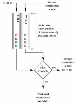
Tokens and buckets
Two
of the key underpinnings of a shaping mechanisms are the interrelated
concepts of tokens and buckets.
In order to control
the rate of dequeuing, an implementation can count the number of packets or
bytes dequeued as each item is dequeued, although this requires complex usage
of timers and measurements to limit accurately. Instead of calculating the
current usage and time, one method, used widely in traffic control, is to
generate tokens at a desired rate, and only dequeue packets or bytes if a token
is available.
Consider
the analogy of an amusement park ride with a queue of people waiting to
experience the ride. Let's imagine a track on which carts traverse a fixed
track. The carts arrive at the head of the queue at a fixed rate. In order to
enjoy the ride, each person must wait for an available cart. The cart is
analogous to a token and the person is analogous to a packet. Again, this
mechanism is a rate-limiting or shaping mechanism. Only a certain number of
people can experience the ride in a particular period.
To
extend the analogy, imagine an empty line for the amusement park ride and a
large number of carts sitting on the track ready to carry people. If a large
number of people entered the line together many (maybe all) of them could
experience the ride because of the carts available and waiting. The number of
carts available is a concept analogous to the bucket. A bucket contains a
number of tokens and can use all of the tokens in bucket without regard for
passage of time.
And
to complete the analogy, the carts on the amusement park ride (our tokens)
arrive at a fixed rate and are only kept available up to the size of the
bucket. So, the bucket is filled with tokens according to the rate, and if the
tokens are not used, the bucket can fill up. If tokens are used the bucket will
not fill up. Buckets are a key concept in supporting bursty traffic such as
HTTP.
The
TBF qdisc is a classical
example of a shaper .The TBF generates rate tokens and only transmits packets when a token is available. Tokens
are a generic shaping concept.
In
the case that a queue does not need tokens immediately, the tokens can be
collected until they are needed. To collect tokens indefinitely would negate
any benefit of shaping so tokens are collected until a certain number of tokens
has been reached. Now, the queue has tokens available for a large number of
packets or bytes which need to be dequeued. These intangible tokens are stored
in an intangible bucket, and the number of tokens that can be stored depends on
the size of the bucket.
This
also means that a bucket full of tokens may be available at any instant. Very
predictable regular traffic can be handled by small buckets. Larger buckets may
be required for burstier traffic, unless one of the desired goals is to reduce
the burstiness of the flows.
In summary, tokens are
generated at rate, and a maximum of a bucket's worth of tokens may be
collected. This allows bursty traffic to be handled, while smoothing and
shaping the transmitted traffic.
The
concepts of tokens and buckets are closely interrelated and are used in both TBF (one of the classless qdiscs) and HTB (one of the classful qdiscs). Within
the tc language, the use of two- and three-color meters is indubitably a
token and bucket concept.
Packets and
frames
The
terms for data sent across network changes depending on the layer the user is
examining. The word frame is typically used to describe a layer 2 (data link)
unit of data to be forwarded to the next recipient. Ethernet interfaces, PPP
interfaces, and T1 interfaces all name their layer 2 data unit a frame. The
frame is actually the unit on which traffic control is performed.
Chapter 2
2.1 Theoretical Basis for Data
Communication
Information can be
transmitted on wires by varying some physical property such as voltage or
current. By representing the value of this voltage or current as a
single-valued function of time, f(t), we can model
the behavior of the signal and analyze it mathematically.
2.1.1 Fourier Analysis
In the early 19th
century, the French mathematician Jean-Baptiste Fourier proved that any
reasonably behaved periodic function, g(t) with period T can be constructed as the sum of a (possibly
infinite) number of sines and cosines:
where f = 1/T is
the fundamental frequency, an and bn are the sine and
cosine amplitudes of the n th harmonics (terms), and c is a constant. Such a
decomposition is called a Fourier series. From the Fourier series, the function can be
reconstructed; that is, if the period, T, is known and the amplitudes
are given, the original function of time can be found by performing the sums of
this eq.
A data signal that
has a finite duration (which all of them do) can be handled by just imagining
that it repeats the entire pattern over and over forever (i.e., the interval
from T
to 2T
is the same as from 0 to T, etc.).
The an
amplitudes can be computed for any given g(t) by multiplying both sides of the
equation by sin(2πkft) and then integrating from 0 to T. Since:
only one term of the summation survives: an.
The bn
summation vanishes completely. Similarly, by multiplying the first equation by cos(2πkft)
and integrating between 0 and T, we can
derive bn.
By just integrating both sides of the equation as it stands, we can find c. The
results of performing these operations are as follows:

2.1.2 Bandwidth limited signals
To see what all this has to do with data communication, let us consider
a specific example: the transmission of the ASCII character ''b'' encoded in an
8-bit byte. The bit pattern that is to be transmitted is 01100010. The
left-hand part of the figure below shows the voltage output by the transmitting
computer. The Fourier analysis of this signal yields the coefficients:
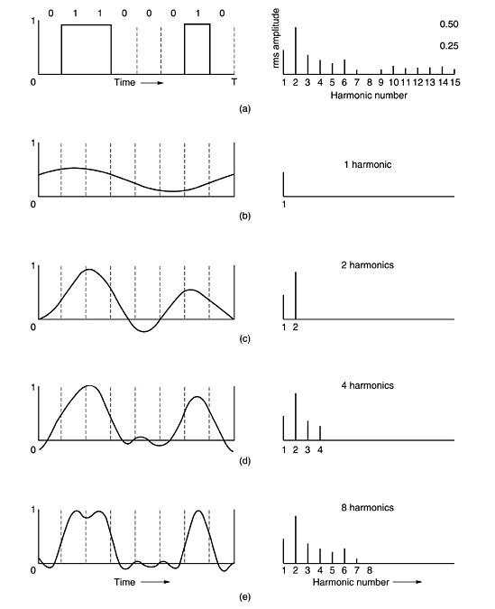
(a) A binary signal and its root-mean-square Fourier
amplitudes.
(b)-(e) Successive approximations to the original signal.


The
root-mean-square amplitudes,  , for the first few terms are shown on the right-hand side of the
figure (a) . These values are of interest because their squares are
proportional to the energy transmitted at the corresponding frequency.
, for the first few terms are shown on the right-hand side of the
figure (a) . These values are of interest because their squares are
proportional to the energy transmitted at the corresponding frequency.
Unfortunately, all
transmission facilities diminish different Fourier components by different
amounts, thus introducing distortion. Usually, the amplitudes are transmitted
undiminished from 0 up to some frequency fc [measured in cycles/sec or Hertz (Hz)] with all frequencies above
this cutoff frequency attenuated. The range of frequencies transmitted without
being strongly attenuated is called the bandwidth.
The bandwidth is a
physical property of the transmission medium and usually depends on the
construction, thickness, and length of the medium.
Now let us consider
how the signal of (a) would look if the bandwidth were so low that only the
lowest frequencies were transmitted [i.e., if the function were being
approximated by the first few terms of the first equation . Figure (b) shows
the signal that results from a channel that allows only the first harmonic (the
fundamental, f)
to pass through. Similarly, fig (c)-(e)
show the spectra and reconstructed functions for higher-bandwidth channels. Limiting the bandwidth limits the data
rate, even for perfect channels.
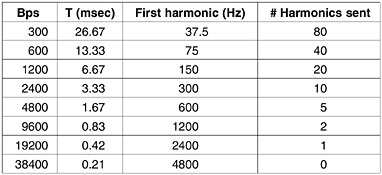
Relation between data rate and
harmonics
As early as 1924,
an AT&T engineer, Henry Nyquist, realized that even a perfect channel has a
finite transmission capacity. He derived an equation expressing the maximum
data rate for a finite bandwidth noiseless channel. In 1948, Claude Shannon
carried Nyquist's work further and extended it to the case of a channel subject
to random (that is, thermodynamic) noise (Shannon, 1948).
Nyquist proved that
if an arbitrary signal has been run through a low-pass filter of bandwidth H, the
filtered signal can be completely reconstructed by making only 2H
(exact) samples per second. Sampling the line faster than 2H times per second is pointless
because the higher frequency components that such sampling could recover have
already been filtered out. If the signal consists of V discrete levels, Nyquist's
theorem states:

For example, a
noiseless 3-kHz channel cannot transmit binary (i.e., two-level) signals at a
rate exceeding 6000 bps.
So far we have
considered only noiseless channels. If random noise is present, the situation
deteriorates rapidly. And there is always random (thermal) noise present due to
the motion of the molecules in the system. The amount of thermal noise present
is measured by the ratio of the signal power to the noise power, called the signal-to-noise
ratio. If we denote the signal power by S and the noise power by N, the
signal-to-noise ratio is S/N. Usually, the ratio itself is not quoted; instead, the
quantity 10  is given. These units are called
decibels
(dB). An S/N
ratio of 10 is 10 dB, a ratio of 100 is 20 dB, a ratio of 1000 is 30 dB, and so
on.
is given. These units are called
decibels
(dB). An S/N
ratio of 10 is 10 dB, a ratio of 100 is 20 dB, a ratio of 1000 is 30 dB, and so
on.
Shannon's major
result is that the maximum data rate of a noisy channel whose bandwidth is H Hz, and
whose signal-to-noise ratio is S/N, is given by:

2.2 . Principles of QoS
Policing
Policers measure
and limit traffic in a particular queue. It can drop or mark traffic
Policing, as an
element of traffic control, is simply a mechanism by which traffic can be
limited. Policing is most frequently used on the network border to ensure that
a peer is not consuming more than its allocated bandwidth. A policer will
accept traffic to a certain rate, and then perform an action on traffic
exceeding this rate. A rather harsh solution is to drop the traffic, although the traffic could be
reclassified instead of being dropped.
A policer is a
yes/no question about the rate at which traffic is entering a queue. If the
packet is about to enter a queue below a given rate, take one action (allow the
enqueuing). If the packet is about to enter a queue above a given rate, take
another action. Although the policer uses a token bucket mechanism internally,
it does not have the capability to delay a packet as a shaping mechanism does.
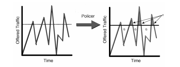
y - temporary bursts permited
only if there are unused tokens G
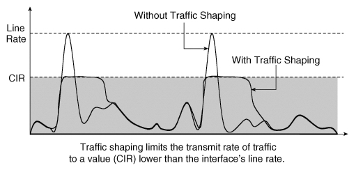
Shaping
Shapers delay
packets to meet a desired rate.
Shaping is the
mechanism by which packets are delayed before transmission in an output queue
to meet a desired output rate. This is one of the most common desires of users
seeking bandwidth control solutions. The act of delaying a packet as part of a
traffic control solution makes every shaping mechanism into a
non-work-conserving mechanism.
Viewed in reverse,
a non-work-conserving queuing mechanism is performing a shaping function. A
work-conserving queuing mechanism would not be capable of delaying a packet.
Shapers attempt to
limit or ration traffic to meet but not exceed a configured rate (frequently
measured in packets per second or bits/bytes per second). As a side effect,
shapers can smooth out bursty traffic. One of the advantages of shaping
bandwidth is the ability to control latency of packets. The underlying
mechanism for shaping to a rate is typically a token and bucket mechanism.
CIR
= Committed information rate, the policed rate
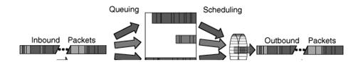
Scheduling
Schedulers arrange
and/or rearrange packets for output.
Scheduling is the mechanism by which packets
are arranged (or rearranged) between input and output of a particular queue. The
overwhelmingly most common scheduler is the FIFO (first-in first-out)
scheduler. From a larger perspective, any set of traffic control mechanisms on
an output queue can be regarded as a scheduler, because packets are arranged
for output.
Other generic scheduling
mechanisms attempt to compensate for various networking conditions. A fair
queuing algorithm (SFQ) attempts to prevent
any single client or flow from dominating the network usage. A round-robin
algorithm gives each flow or client a
turn to dequeue packets. Other sophisticated scheduling algorithms attempt to
prevent backbone overload (GRED) or refine other
scheduling mechanisms (ESFQ).
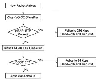
Classifying
Classifiers sort or
separate traffic into queues in other words the selection of traffic.
Classifying is the
mechanism by which packets are separated for different treatment, possibly
different output queues. During the process of accepting, routing and
transmitting a packet, a networking device can classify the packet a number of
different ways. Classification can include marking the packet, which usually happens on
the boundary of a network under a single administrative control or
classification can occur on each hop individually.
The Linux model allows for a packet to cascade
across a series of classifiers in a traffic control structure and to be
classified in conjunction with policers.
Dropping
Dropping discards
an entire packet, flow or classification.
Dropping a packet
is a mechanism by which a packet is discarded.
Marking
Marking is a
mechanism by which the packet is altered.
2.3 Kernel options and packages neeed
for traffic shaping
2.3.1 Kernel compilation options
If you've never setup traffic
shaping before, you'll need to enable traffic shaping, and check if your linux
has routing capabilites, too. Moreover, you'll need to enable netfilter support
for iptables if you haven't set that up yet, either.
The options listed below are taken from a
2.4.33.3 kernel source tree. If you
don't have the sources take your time and get them from www.kernel.org . I'm using a 2.4 kernel just
because it's rock-solid on Slackware/Debian and a lot of people will run 2.4
kernel for a long time to come and some of the changes to the system in a 2.6
kernel aren't necesarly to 2.4. The 2.6 kernel series shows a great deal of
improvment but it's still undergoing
heavy development and the stability of any given release can be
hit-or-miss.
Below are the options for setting your linux
box to forward packets (routing). The exact options may differ slightly from
kernel release to kernel release depending on patches and new schedulers and
classifiers.
The selections for
forwarding traffic on 2.6 series kernel are listed under Networking -> Networking
options
Networking options --->
<*>
Packet socket
[*] Packet socket: mmapped IO
<*> Netlink device
emulation
[*] Network packet filtering
(replaces ipchains)
[*] Socket Filtering
<*> Unix domain
sockets
[*] TCP/IP networking
[*] IP:
multicasting
[*] IP: advanced router
[*] IP: policy routing
[*] IP: use netfilter MARK value as routing
key
[*] IP: fast network address
translation
[*] IP: equal cost multipath
[*] IP: use TOS value as routing key
[*] IP: verbose route monitoring
[ ] IP: kernel level autoconfiguration
< > IP: tunneling
< > IP: GRE tunnels over IP
[ ] IP: multicast routing
[ ] IP: ARP daemon support (EXPERIMENTAL)
[ ] IP: TCP Explicit Congestion Notification
support
[*] IP: TCP syncookie support (disabled per
default)
Next step is to
enable the flow classifiers. You will need to enable th options selected below
to use Netfilter effectively to classify traffic flows and fou use for
firewalling, too
The selections for
Netfilter for a 2.6 series kernel are listed under Networking -> Networking
options -> Network packet filtering (replaces ipchains) -> IP: Netfilter
Configuration..
Networking options ---> IP:
Netfilter Configuration --->
<M>
Connection tracking (required for masq/NAT)
<M> Userspace queueing
via NETLINK
<M> IP tables support
(required for filtering/masq/NAT)
<M> limit match support
<M> IPP2P match support
<M> MAC address match support
<M> Packet type match support
<M> netfilter MARK match support
<M> Multiple port match support
<M> TOS match support
<M> recent match support
<M> ECN match support
<M> DSCP match support
<M> AH/ESP match support
<M> LENGTH match support
<M> TTL match support
<M> tcpmss match support
<M> stealth match support
<M> Unclean match support
<M> Owner match support
<M> Packet filtering
<M> REJECT target support
<M> MIRROR target support
<M> Packet mangling
<M> TOS target support
<M> ECN target support
<M> DSCP target support
<M> MARK target support
<M> LOG target support
<M> ULOG target support
<M> TCPMSS target support
<M> ARP tables
support
<M> ARP packet filtering
<M> ARP payload mangling
< > ipchains (2.2-style)
support
< > ipfwadm (2.0-style)
support
For classifing p2p
traffic I prefer to use the extension of iptables
called IPP2P. This is obtained by patching the actual surce code of the kernel
with the patch-o-matic-ng obtained
from https://ftp.netfilter.org/pub/patch-o-matic-ng/snapshot/ .
Now
it's time for enabling the traffic
control support . Many distributions provide kernels with modular or monolithic
support for traffic control (Quality of Service). Custom kernels may not
already provide support (modular or not).
The selections for
traffic control for a 2.6 series kernel are listed under Networking -> Networking
options -> QoS and/or fair queuing.
At a minimum you will want to enable the options selected below.
[*] QoS and/or fair
queueing
<M> CBQ packet scheduler
<M> HTB packet scheduler
<M> CSZ packet scheduler
<M> H-FSC packet scheduler
<M> The simplest PRIO pseudoscheduler
<M> RED queue
<M> SFQ queue
<M> TEQL queue
<M> TBF queue
<M> GRED queue
<M> Network emulator
<M> Diffserv field marker
<M> Ingress Qdisc
[*] QoS support
[*] Rate estimator
[*] Packet classifier API
<M> TC index classifier
<M> Routing table based classifier
<M> Firewall based classifier
<M> U32 classifier
<M> Special RSVP classifier
<M> Special RSVP classifier for IPv6
[*] Traffic policing (needed for
in/egress)
2.3.2 Netfilter iptables
Netfilter is a very important part of the Linux kernel in
terms of security, packet mangling, and manipulation. The front end for
netfilter is iptables, which 'tells' the kernel what the user wants
to do with the IP packets arriving into, passing through, or leaving the Linux
box.
The most used features of netfilter are packet
filtering and network address translation, but there are a lot of other things
that we can do with netfilter, such as packet mangling Layer 7 filtering. It can be obtained from ftp://ftp.netfilter.org/pub/iptables/
Optionally we need patch-o-matic-ng for adding the IPP2P extension. The goal of the IPP2P
is to identify peer-to-peer (P2P) data in IP traffic. Thereby IPP2P integrates
itself easily into existing Linux firewalls and it's functionality can be used
by adding appropriate filter rules. It can be obtained from https://www.ipp2p.org/
Netfilter has a few tables, each containing a default
set of rules, which are called chains. The default table loaded into the kernel
is the filter table, which contains three chains:
INPUT: Contains rules for packets destined to the Linux
machine itself.
FORWARD: Contains rules for packets that the Linux machine
routes to another IP address.
OUTPUT: Contains rules for packets generated by the Linux
machine.
The operations iptables can do
with chains are:
List the rules
in a chain (iptables -L CHAIN).
Change the policy
of a chain (iptables -P CHAIN ACCEPT).
Create a new
chain (iptables -N CHAIN).
Flush a chain;
delete all rules (iptables -F CHAIN).
Delete a chain
(iptables -D CHAIN), only if the
chain is empty.
Zero counters
in a chain (iptables -Z CHAIN). Every
rule in every chain keeps a counter of the number of packets and bytes it
matched. This command resets those counters.
For the -L, -F, -D, and -Z operations, if the chain name is
not specified, the operation is applied to the entire table, which if not
specified is by default the filter table. To specify the table on which we do
operations, we must use the -t switch like so iptables -t filter .
Operations that
iptables can execute on rules are:
Append rules to
a chain (iptables -A)
Insert rules in
a chain (iptables -I)
Replace a rule
from a chain (iptables -R)
Delete a rule
from a chain (iptables -D)
During run
time, you will prefer to use -I more
than -A because often you need to
insert temporary rules in the chain while iptables
-A places the rule at the end of the chain, while iptables -I places the rule on the top of the other rules in the
chain. However, you can insert a rule anywhere in the chain by specifying the
position where you want the rule to be in the chain with the -I switch:
iptables
-I CHAIN 4 will insert a rule at the fourth position of the specified
chain.
2.3.3 iproute2 tools (tc)
Iproute2 is
a suite of command line utilities which manipulate kernel structures for IP
networking configuration on a machine. Of the tools in the iproute2 package,
the binary tc is the only one used for traffic control . Because it interacts
with the kernel to direct the creation, deletion and modification of traffic
control structures, the tc binary needs to be compiled with support for all of
the qdiscs you wish to use. In particular, the HTB qdisc is not supported yet
in the upstream iproute2 package .
It can be obtained
from https://developer.osdl.org/dev/iproute2/
The ip
tool provides most of the networking configuration a Linux box needs. You can
configure interfaces, ARP, policy routing, tunnels, etc.
Now, with IPv4
and IPv6, ip can do pretty much anything (including a lot that we don't need in
our particular situations). The syntax of ip is not difficult, and there is a
lot of documentation on this subject. However, the most important thing is
knowing what we need and when we need it.
Let's have a look at the ip
command help to see what ip knows:
# ip help
Usage: ip [ OPTIONS ]
OBJECT
ip [ -force ] [-batch filename
where OBJECT :=
OPTIONS := |
-o[neline] | -t[imestamp] }
The ip link command shows the network
device's configurations that can be changed with ip link set. This command is used to modify the device's
proprieties and not the IP address.
The IP
addresses can be configured using the ip
addr command. This command can be used to add a primary or secondary
(alias) IP address to a network device (ip
addr add), to display the IP addresses for each network device (ip addr show), or to delete IP addresses
from interfaces (ip addr del). IP
addresses can also be flushed using different criteria, e.g. ip addr flush dynamic will flush all
routes added to the kernel by a dynamic routing protocol.
Neighbor/Arp
table management is done using ip
neighbor, which has a few commands expressively named add, change, replace, delete, and flush.
ip tunnel is used to manage tunneled connections. Tunnels can be gre, ipip, and sit.
The ip tool offers a way for monitoring
routes, addresses, and the states of devices in real-time. This can be
accomplished using ip monitor, rtmon, and rtacct commands included in the iproute2 package.
One very
important and probably the most used object of the ip tool is ip route, which can do any operations on
the kernel routing table. It has commands to add, change, replace, delete,
show, flush, and get routes.
One of the
things iproute2 introduced to Linux that ensured its popularity was policy
routing. This can be done using ip rule
and ip route in a few simple steps.
The tc command allows administrators to build different QoS
policies in their networks using Linux instead of very expensive dedicated QoS
machines. Using Linux, you can implement QoS in all the ways any dedicated QoS
machine can and even more. Also, one can make a bridge using a good PC running
Linux that can be transformed into a very powerful and very cheap dedicated QoS
machine.
2.4 Queueing disciplines for
bandwidth management
To prevent confusion, tc uses the following
rules for bandwith specification:
mbps = 1024 kbps = 1024 * 1024 bps => byte/s
mbit = 1024 kbit => kilo bit/s.
mb = 1024 kb = 1024 * 1024 b => byte
mbit = 1024 kbit => kilo bit.
but when it prints out the rates it will use:
1Mbit = 1024 Kbit = 1024 * 1024 bps => byte/s
With queueing we
determine the way in which data is SENT. It is important to realise that we can
only shape data that we transmit.
With the way the
Internet works, we have no direct control of what people send us. However, the Internet
is mostly based on TCP/IP which has a few features that help us. TCP/IP has no
way of knowing the capacity of the network between two hosts, so it just starts
sending data faster and faster ('slow start') and when packets start getting
lost, because there is no room to send them, it will slow down. In fact it is a
bit smarter than this, but more about that later.
If you have a
router and wish to prevent certain hosts within your network from downloading
too fast, you need to do your shaping on the *inner* interface of your router,
the one that sends data to your own computers.
You also have to be
sure you are controlling the bottleneck of the link. If you have a 100Mbit NIC
and you have a router that has a 256kbit link, you have to make sure you are
not sending more data than your router can handle. Otherwise, it will be the
router who is controlling the link and shaping the available bandwith. We need
to 'own the queue' so to speak, and be the slowest link in the chain. Luckily
this is easily possible.
As said, with
queueing disciplines, we change the way data is sent. Classless queueing disciplines are those that, by and large accept data
and only reschedule, delay or drop it.
These can be used to shape traffic for an
entire interface, without any subdivisions. It is vital that you understand
this part of queueing before we go on the classful qdisc-containing-qdiscs!
Each of these
queues has specific strengths and weaknesses and can be used as the primary
qdisc on an interface or can be used inside a leaf class of a classfull qdiscs.
Not all of them may be as well tested.
The Linux traffic
shaping implementation allows you to build arbitrarily complicated
configurations, based upon the building block of the qdisc. You can choose from
two kinds of qdiscs: classless and classful. By default, all Ethernet
interfaces get a classless qdisc for free, which is essentially a FIFO. You
will likely replace this with something more interesting. Classful qdiscs, on
the other hand, can contain classes to arbitrary levels of depth. Leaf classes,
those which are not parents of additional classes, hold a default FIFO style
qdisc. Classless qdiscs are schedulers. Classful qdiscs are generally shapers,
but some schedule as well.
Each network
interface effectively has two places where you can attach qdiscs: root and
ingress. root is essentially a synonym for egress. The distinction between
these two hooks into Linux QoS is essential. The root hook sits on the inside
of your Ethernet interface. You can effectively apply traffic classification
and scheduling against the root hook as any queue you create is under your
control. The ingress hook rests on the outside of your Ethernet interface. You
cannot shape this traffic, but merely throttle it, because it has already
arrived.
2.4.1
Classless Queuing Disciplines (qdiscs)
Lets consider the
example below:
tc qdisc add dev eth2 parent
root handle 1:0 pfifo
First, we specify
that we want to work with a qdisc.
Next, we indicate we wish to add a
new qdisc to the Ethernet device eth2.
(You can specify del in place of add to remove the qdisc in question.)
Then, we specify the special parent root.
It is the hook on the egress side of your Ethernet interface. The handle is the magic userspace way of
naming a particular qdisc, but more on that later. Finally, we specify the
qdisc we wish to add. Because pfifo
is a classless qdisc, there is nothing more to do.
Qdiscs are always
referred to using a combination of a major node number and a minor node number.
For any given qdisc, the major node number has to be unique for the root hook
for a given Ethernet interface. The minor number for any given qdisc will
always be zero. By convention, the first qdisc created is named 1:0. You could,
however, choose 7:0 instead. These numbers are actually in hexadecimal, so any
values in within the range of 1 to ffff are also valid. For readability the
digits 0 to 9 are generally used exclusively.
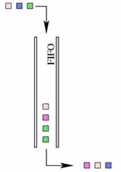
2.4.1.1 FIFO, First-In First-Out
(pfifo and bfifo)
The FIFO algorithm forms the basis
for the default qdisc on all Linux network interfaces (pfifo_fast). It performs
no shaping or rearranging of packets. It simply transmits packets as soon as it
can after receiving and queuing them. This is also the qdisc used inside all
newly created classes until another qdisc or a class replaces the FIFO.
A FIFO qdisc must, however, have a size limit (a buffer size) to prevent
it from overflowing in case it is unable to dequeue packets as quickly as it
receives them. Linux implements two basic FIFO qdiscs, one based on bytes, and
one on packets. Regardless of the type of FIFO used, the size of the queue is
defined by the parameter limit. For a pfifo the unit is understood to be
packets and for a bfifo the unit is understood to be bytes.
tc
qdisc add dev eth0 handle 1:0 root dsmark indices 1 default_index 0
tc
qdisc add dev eth0 handle 2:0 parent 1:0 pfifo limit 30
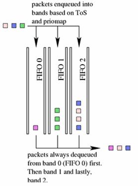
2.4.1.2 pfifo_fast,
the default Linux qdisc
The pfifo_fast qdisc is the default qdisc for
all interfaces under Linux. Based on a conventional FIFO qdisc, this qdisc also
provides some prioritization. It provides three different bands (individual
FIFOs) for separating traffic. The highest priority traffic (interactive flows)
are placed into band 0 and are always serviced first. Similarly, band 1 is
always emptied of pending packets before band 2 is dequeued.
There is nothing configurable to the
end user about the pfifo_fast qdisc
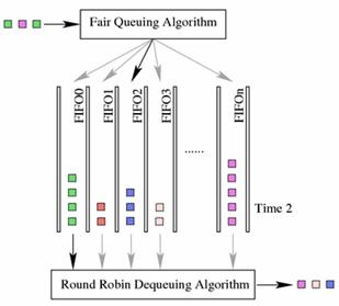
2.4.1.3 SFQ,
Stochastic Fair Queuing
The SFQ qdisc attempts to fairly distribute opportunity to transmit data
to the network among an arbitrary number of flows. It accomplishes this by
using a hash function to separate the traffic into separate (internally
maintained) FIFOs which are dequeued in a round-robin fashion. Because there is
the possibility for unfairness to manifest in the choice of hash function, this
function is altered periodically. Perturbation (the parameter perturb) sets
this periodicity.
tc qdisc add dev eth0 handle 1:0
root dsmark indices 1 default_index 0
tc qdisc add dev eth0 handle 2:0
parent 1:0 sfq perturb 10
2.4.1.4 Other
classless qdiscs (ESFQ,GRED,TBF)
ESFQ, Extended Stochastic Fair Queuing
Conceptually, this qdisc is no different than
SFQ although it allows the user to control more parameters than its simpler
cousin. This qdisc was conceived to overcome the shortcoming of SFQ identified
above. By allowing the user to control which hashing algorithm is used for
distributing access to network bandwidth, it is possible for the user to reach
a fairer real distribution of bandwidth.
tc qdisc add dev eth0 root esfq
perturb 10
GRED, Generic Random Early Drop
Theory declares that a RED algorithm is useful on a backbone or core
network with data rates over 100 Mbps, but not as useful near the end-user
TBF, Token Bucket Filter
This qdisc is built on tokens and buckets. It simply shapes traffic
transmitted on an interface. To limit the speed at which packets will be
dequeued from a particular interface, the TBF qdisc is the perfect solution. It
simply slows down transmitted traffic to the specified rate. Packets are only transmitted if there are
sufficient tokens available. Otherwise, packets are deferred. Delaying packets
in this fashion will introduce an artificial latency into the packet's round
trip time.
tc qdisc add dev eth0 handle 1:0
root dsmark indices 1 default_index 0
tc qdisc add dev eth0 handle 2:0
parent 1:0 tbf burst 20480 limit 20480 mtu 1514 rate 32000bps
2.4.2 Classfull qdisc
Now, let us look at
an example where we add a classful qdisc and a single class.
# tc qdisc add dev eth2 parent
root handle 1:0 htb default 1
# tc class add dev eth2
parent 1:0 classid 1:1 htb rate 1mbit
The first line
seams to be almost identical to the previous classless qdisc. Here we used the htb qdisc. The parameter default it is an option for htb qdiscs
In the second line
we use the tc binary with the class argument, instead of the qdisc argument. The class argument allows you to create a
class hierarchy. We are working with Ethernet device eth2 again. The parent parameter enables you to attach
this class to either an existing classful qdisc or another class of the same
type. Above we attach to the htb
qdisc we just attached to the root hook earlier.
The value for the parent parameter must be the major and
minor node number of the qdisc or class you wish to attach to. Earlier, the
identifier 1:0 was chosen for handle of
the htb qdisc. That must be used as
the argument to the parent parameter
so tc knows where you are assigning
this class.
The classid parameter serves the same
purpose for classes that the handle
parameter serves for qdiscs. It is the identifier for this specific class. The
major node number has already been chosen for you. It must be the same as the
major node number specified for the parent
argument earlier. You are free to choose any minor node number you want for the
classid parameter. Traditionally
numbering starts at 1, but numbers from 1 to ffff are valid. For this class the
classid 1:1 was chosen, because the
qdisc it is being attached to has a major node number 1 for its handle parameter.
Finally we specify
the type of class and any options that class requires. In this instance, the
htb class was chosen, as the htb qdisc can only have htb classes assigned to
it. (This is generally true of classful qdiscs.)
A
combined example using both classfull and classless qdiscs.
# tc qdisc add dev eth2
parent root handle 1:0 htb default 20
# tc class add dev eth2
parent 1:0 classid 1:1 htb rate 1000kbit
# tc class add dev eth2
parent 1:1 classid 1:10 htb rate 500kbit
# tc class add dev eth2
parent 1:1 classid 1:20 htb rate 500kbit
# tc qdisc add dev eth2
parent 1:20 handle 2:0 sfq
Now we have a
nested structure, with a htb classful qdisc assigned to the root hook, three
htb classes, and asfq qdisc as a leaf qdisc for one htb class. The other has an
implicit pfifo attached. The careful reader will notice each qdisc has a minor
node number of zero, as is required.
A graphical
representation of the class hierarchy just created should be beneficial.
First, notice the
at the top of the hierarchy is a htb
qdisc. Three classes are assigned to it. Only the first is immediately attached
to it, using the parent 1:0. The
other two classes are children of the first class. If you examine the tc command with the class option, you will see that the parent refers to the parent class in
the hierarchy via its classid.
Each of the three htb classes attached to the htb qdisc are assigned a major node
number of 1 for the classid, as the
qdisc they are attached to has a handle
with 1 as the major node number.
Finally, a sfq qdisc is attached to the leaf class
with classid 1:20. Notice the qdisc
is added nearly the same as the htb.
However, instead of being assigned to the magic root hook, the target is 1:20. The handle is chosen based on the rules discussed earlier
This whole structure can be deleted simply by
deleting the root hook as demonstrated below.
# tc qdisc del dev eth2 root
Displaying qdisc and class Details
Now we can take a
look at the details of the hierarchy we have created. Using the tc tool again
the following output is produced.
# tc -s -d qdisc show dev
eth2
qdisc sfq 2: quantum 1514b
limit 128p flows 128/1024
Sent 0 bytes 0 pkts (dropped 0, overlimits 0)
qdisc htb 1: r2q 10 default 0
direct_packets_stat 0 ver 3.16
Sent 0 bytes 0 pkts (dropped 0, overlimits 0)
Each qdisc in your
hierarchy is shown along with statistics and the details of its parameters. The
information available for each qdisc varies. The number of sent bytes and
packets is self explanatory. For classful qdiscs, the totals are class wide and
include the dequeue totals from children and siblings.
# tc -s -d class show dev
eth2
class htb 1:10 root leaf 2:
prio 0 quantum 13107 rate 1Mbit ceil 1Mbit
burst 2909b/8 mpu 0b cburst 2909b/8 mpu 0b
level 0
Sent 0 bytes 0 pkts (dropped 0, overlimits 0)
lended: 0 borrowed: 0 giants: 0
tokens: 28791 ctokens: 2879
The detailed output
for classes is similar to that of qdiscs. The information available varies
depending on the type of class. The above is typical of a htb qdisc's class.
2.4.2.1 HTB,
Hierarchical Token Bucket
HTB uses the concepts of tokens and buckets along with the class-based
system and filters to allow for complex and granular control over traffic. With
a complex borrowing model, HTB can perform a variety of sophisticated traffic
control techniques. One of the easiest ways to use HTB immediately is that of
shaping.
By understanding tokens and buckets or by grasping the function of TBF,
HTB should be merely a logical step. This queuing discipline allows the user to
define the characteristics of the tokens and bucket used and allows the user to
nest these buckets in an arbitrary fashion. When coupled with a classifying
scheme, traffic can be controlled in a very granular fashion.
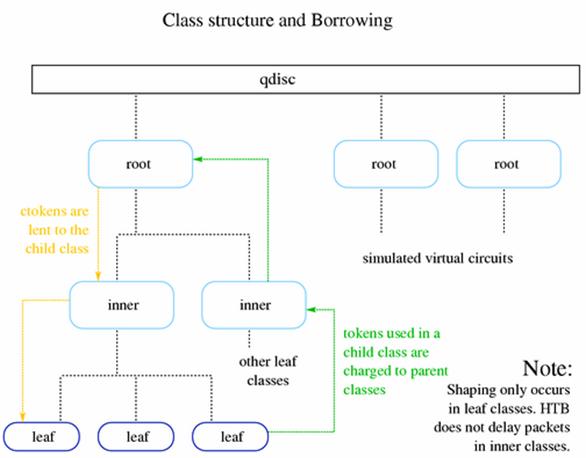
A fundamental part of the HTB qdisc is the borrowing mechanism. Children
classes borrow tokens from their parents once they have exceeded rate. A child
class will continue to attempt to borrow until it reaches ceil, at which point
it will begin to queue packets for transmission until more tokens/ctokens are
available. As there are only two primary types of classes which can be created
with HTB the following table and diagram identify the various possible states
and the behaviour of the borrowing mechanisms.
HTB class states and potential actions taken
|
type of class
|
class state
|
HTB internal state
|
action taken
|
|
leaf
|
< rate
|
HTB_CAN_SEND
|
Leaf class will dequeue queued
bytes up to available tokens (no more than burst packets)
|
|
leaf
|
> rate, < ceil
|
HTB_MAY_BORROW
|
Leaf class will attempt to borrow
tokens/ctokens from parent class. If tokens are available, they will be lent
in quantum increments and the leaf class will dequeue up to cburst bytes
|
|
leaf
|
> ceil
|
HTB_CANT_SEND
|
No packets will be
dequeued. This will cause packet delay and will increase latency to meet the
desired rate.
|
|
inner, root
|
< rate
|
HTB_CAN_SEND
|
Inner class will lend tokens to
children.
|
|
inner, root
|
> rate, < ceil
|
HTB_MAY_BORROW
|
Inner class will
attempt to borrow tokens/ctokens from parent class, lending them to competing
children in quantum increments per request.
|
|
inner, root
|
> ceil
|
HTB_CANT_SEND
|
Inner class will not attempt to
borrow from its parent and will not lend tokens/ctokens to children classes.
|
This diagram identifies the flow of borrowed tokens and the manner in
which tokens are charged to parent classes. In order for the borrowing model to
work, each class must have an accurate count of the number of tokens used by
itself and all of its children. For this reason, any token used in a child or
leaf class is charged to each parent class until the root class is reached.
Any child class which wishes to borrow a token will request a token from
its parent class, which if it is also over its rate will request to borrow from
its parent class until either a token is located or the root class is reached.
So the borrowing of tokens flows toward the leaf classes and the charging of
the usage of tokens flows toward the root class.
HTB class parameters
default - An optional parameter with every HTB qdisc object, the default default
is 0, which cause any unclassified traffic to be dequeued at hardware speed,
completely bypassing any of the classes attached to the root qdisc.
rate - Used to set the minimum desired speed to which to limit transmitted
traffic. This can be considered the equivalent of a committed information rate
(CIR), or the guaranteed bandwidth for a given leaf class.
ceil - Used to set the maximum desired speed to which to limit the transmitted
traffic. The borrowing model should illustrate how this parameter is used. This
can be considered the equivalent of "burstable bandwidth".
burst - This is the size of the rate bucket HTB will dequeue burst bytes before
awaiting the arrival of more tokens.
cburst - This is the size of the ceil bucket . HTB will dequeue cburst bytes
before awaiting the arrival of more ctokens.
quantum - This is a key parameter used by HTB to control borrowing. Normally, the
correct quantum is calculated by HTB, not specified by the user. Tweaking this
parameter can have tremendous effects on borrowing and shaping under
contention, because it is used both to split traffic between children classes
over rate (but below ceil) and to transmit packets from these same classes.
r2q - Also, usually calculated for the user, r2q is a hint to HTB to help
determine the optimal quantum for a particular class.
mpu -The Minimum Packet Unit
determines the minimal token usage for a packet
MPU=64 # Ethernet
MPU=106 # suited for
DSL users
prio - This is the priority of each class of borrowing from the parent class .
The class with the highest prio value is queued first
2.4.2.2 Other classfull qdiscs (CBQ HFSC PRIO
CBQ, Class Based Queuing
CBQ is the classic
implementation (also called venerable) of a traffic control system.
HFSC, Hierarchical Fair Service Curve
The HFSC classful qdisc balances delay-sensitive traffic against
throughput sensitive traffic. In a congested or backlogged state, the HFSC
queuing discipline interleaves the delay-sensitive traffic when required
according service curve definitions
PRIO, priority scheduler
The PRIO
classful qdisc works on a very simple precept. When it is ready to dequeue a
packet, the first class is checked for a packet. If there's a packet, it gets
dequeued. If there's no packet, then the next class is checked, until the
queuing mechanism has no more classes to check.
2.5 IPv4 variable reference (kernel parameters)
Reverse path filtering
By default, routers route everything, even packets which 'obviously' don't
belong on your network. A common example is private IP space escaping onto the
Internet. If you have an interface with a route of 194.82.28.0/24 to it, you do
not expect packets from 212.93.136.1 to arrive there.
Lots of people will want to turn this feature off, so the kernel hackers
have made it easy. There are files in /proc where you can tell the kernel to do
this for you. The method is called 'Reverse Path Filtering'.
Basically, if the reply to a packet wouldn't go out the interface this packet came
in, then this is a bogus packet and should be ignored.
The following fragment
will turn this on for all current and future interfaces.
# for i in
/proc/sys/net/ipv4/conf/*/rp_filter ; do
> echo 2 > $i
> done
Going by the example above, if a packet arrived on the Linux router on
eth1 claiming to come from the Office+ISP subnet, it would be dropped.
Similarly, if a packet came from the Office subnet, claiming to be from
somewhere outside your firewall, it would be dropped also.
The above is full reverse path filtering. The default is to only filter
based on IPs that are on directly connected networks. This is because the full
filtering breaks in the case of asymmetric routing (where packets come in one
way and go out another, like satellite traffic, or if you have dynamic (bgp,
ospf, rip) routes in your network. The data comes down through the satellite
dish and replies go back through normal land-lines).
If this exception applies to you (and you'll probably know if it does)
you can simply turn off the rp_filter on the interface where the satellite data
comes in. If you want to see if any packets are being dropped, the log_martians
file in the same directory will tell the kernel to log them to your syslog.
# echo 1
>/proc/sys/net/ipv4/conf/all/log_martians
Or
# echo 1
>/proc/sys/net/ipv4/conf/<device_name>/log_martians
Generic ipv4
(https://ipsysctl-tutorial.frozentux.net/chunkyhtml/variablereference.html)
Most rate limiting features don't work on loopback, so don't test them
locally. The limits are supplied in 'jiffies', and are enforced using the
earlier mentioned token bucket filter.
The kernel has an internal clock which runs at 'HZ' ticks (or 'jiffies')
per second. On Intel, 'HZ' is mostly 100. So setting a *_rate file to, say 50,
would allow for 2 packets per second. The token bucket filter is also
configured to allow for a burst of at most 6 packets, if enough tokens have
been earned.
/proc/sys/net/ipv4/icmp_destunreach_rate - If the kernel decides that it can't deliver a
packet, it will drop it, and send the source of the packet an ICMP notice to
this effect.
/proc/sys/net/ipv4/icmp_echo_ignore_all - Don't act on echo packets at all. Please don't
set this by default, but if you are used as a relay in a DoS attack, it may be
useful.
/proc/sys/net/ipv4/icmp_echo_ignore_broadcasts - If you ping the broadcast address of a
network, all hosts are supposed to respond. This makes for a dandy
denial-of-service tool. Set this to 1 to ignore these broadcast messages.
/proc/sys/net/ipv4/icmp_echoreply_rate - The rate at which echo replies are sent to any
one destination.
/proc/sys/net/ipv4/icmp_ignore_bogus_error_responses
- Set this to ignore ICMP
errors caused by hosts in the network reacting badly to frames sent to what
they perceive to be the broadcast address.
/proc/sys/net/ipv4/icmp_paramprob_rate - A relatively unknown ICMP message, which is
sent in response to incorrect packets with broken IP or TCP headers. With this
file you can control the rate at which it is sent.
/proc/sys/net/ipv4/icmp_timeexceed_rate - This is the famous cause of the 'Solaris middle
star' in traceroutes. Limits the rate of ICMP Time Exceeded messages sent.
/proc/sys/net/ipv4/igmp_max_memberships -Maximum number of listening igmp (multicast)
sockets on the host. FIXME: Is this true?
/proc/sys/net/ipv4/inet_peer_gc_maxtime - Add a little explanation about the inet peer
storage? Miximum interval between garbage collection passes. This interval is
in effect under low (or absent) memory pressure on the pool. Measured in jiffies.
/proc/sys/net/ipv4/inet_peer_gc_mintime - Minimum interval between garbage collection
passes. This interval is in effect under high memory pressure on the pool.
Measured in jiffies.
/proc/sys/net/ipv4/inet_peer_maxttl - Maximum time-to-live of entries. Unused entries
will expire after this period of time if there is no memory pressure on the
pool (i.e. when the number of entries in the pool is very small). Measured in
jiffies.
/proc/sys/net/ipv4/inet_peer_minttl - Minimum time-to-live of entries. Should be
enough to cover fragment time-to-live on the reassembling side. This minimum
time-to-live is guaranteed if the pool size is less than inet_peer_threshold.
Measured in jiffies.
/proc/sys/net/ipv4/inet_peer_threshold - The approximate size of the INET peer storage.
Starting from this threshold entries will be thrown aggressively. This
threshold also determines entries' time-to-live and time intervals between
garbage collection passes. More entries, less time-to-live, less GC interval.
/proc/sys/net/ipv4/ip_autoconfig - This file contains the number one if the host
received its IP configuration by RARP, BOOTP, DHCP or a similar mechanism.
Otherwise it is zero.
/proc/sys/net/ipv4/ip_default_ttl - Time To Live of packets. Set to a safe 64.
Raise it if you have a huge network. Don't do so for fun - routing loops cause
much more damage that way. You might even consider lowering it in some
circumstances.
/proc/sys/net/ipv4/ip_dynaddr - You need to set this if you use dial-on-demand
with a dynamic interface address. Once your demand interface comes up, any
local TCP sockets which haven't seen replies will be rebound to have the right
address. This solves the problem that the connection that brings up your
interface itself does not work, but the second try does.
/proc/sys/net/ipv4/ip_forward - If the kernel should attempt to forward
packets. Off by default.
/proc/sys/net/ipv4/ip_local_port_range - Range of local ports for outgoing connections.
Actually quite small by default, 1024 to 4999.
/proc/sys/net/ipv4/ip_no_pmtu_disc - Set this if you want to disable Path MTU
discovery - a technique to determine the largest Maximum Transfer Unit possible
on your path. See also the section on Path MTU discovery in the Cookbook
chapter.
/proc/sys/net/ipv4/ipfrag_high_thresh - Maximum memory used to reassemble IP fragments.
When ipfrag_high_thresh bytes of memory is allocated for this purpose, the
fragment handler will toss packets until ipfrag_low_thresh is reached.
/proc/sys/net/ipv4/ip_nonlocal_bind - Set this if you want your applications to be
able to bind to an address which doesn't belong to a device on your system.
This can be useful when your machine is on a non-permanent (or even dynamic)
link, so your services are able to start up and bind to a specific address when
your link is down.
/proc/sys/net/ipv4/ipfrag_low_thresh - Minimum memory used to reassemble IP fragments.
/proc/sys/net/ipv4/ipfrag_time - Time in seconds to keep an IP fragment in
memory.
/proc/sys/net/ipv4/tcp_abort_on_overflow - A boolean flag controlling the behaviour under
lots of incoming connections. When enabled, this causes the kernel to actively
send RST packets when a service is overloaded.
/proc/sys/net/ipv4/tcp_fin_timeout - Time to hold socket in state FIN-WAIT-2, if it
was closed by our side. Peer can be broken and never close its side, or even
died unexpectedly. Default value is 60sec. Usual value used in 2.2 was 180
seconds, you may restore it, but remember that if your machine is even
underloaded WEB server, you risk to overflow memory with kilotons of dead
sockets, FIN-WAIT-2 sockets are less dangerous than FIN-WAIT-1, because they
eat maximum 1.5K of memory, but they tend to live longer. Cf. tcp_max_orphans.
/proc/sys/net/ipv4/tcp_keepalive_time - How often TCP sends out keepalive messages when
keepalive is enabled. Default: 2hours.
/proc/sys/net/ipv4/tcp_keepalive_intvl - How frequent probes are retransmitted, when a
probe isn't acknowledged. Default: 75 seconds.
/proc/sys/net/ipv4/tcp_keepalive_probes - How many keepalive probes TCP will send, until
it decides that the connection is broken. Default value: 9. Multiplied with
tcp_keepalive_intvl, this gives the time a link can be non-responsive after a
keepalive has been sent.
/proc/sys/net/ipv4/tcp_max_orphans - Maximal number of TCP sockets not attached to
any user file handle, held by system. If this number is exceeded orphaned
connections are reset immediately and warning is printed. This limit exists
only to prevent simple DoS attacks, you _must_ not rely on this or lower the
limit artificially, but rather increase it (probably, after increasing
installed memory), if network conditions require more than default value, and
tune network services to linger and kill such states more aggressively. Let me
remind you again: each orphan eats up to 64K of unswappable memory.
/proc/sys/net/ipv4/tcp_orphan_retries - How may times to retry before killing TCP
connection, closed by our side. Default value 7 corresponds to 50sec-16min depending on RTO. If your machine
is a loaded WEB server, you should think about lowering this value, such
sockets may consume significant resources. Cf. tcp_max_orphans.
/proc/sys/net/ipv4/tcp_max_syn_backlog - Maximal number of remembered connection
requests, which still did not receive an acknowledgment from connecting client.
Default value is 1024 for systems with more than 128Mb of memory, and 128 for
low memory machines. If server suffers of overload, try to increase this
number. Warning! If you make it greater than 1024, it would be better to change
TCP_SYNQ_HSIZE in include/net/tcp.h to keep
TCP_SYNQ_HSIZE*16<=tcp_max_syn_backlog and to recompile kernel.
/proc/sys/net/ipv4/tcp_max_tw_buckets - Maximal number of timewait sockets held by
system simultaneously. If this number is exceeded time-wait socket is
immediately destroyed and warning is printed. This limit exists only to prevent
simple DoS attacks, you _must_ not lower the limit artificially, but rather
increase it (probably, after increasing installed memory), if network
conditions require more than default value.
/proc/sys/net/ipv4/tcp_retrans_collapse - Bug-to-bug compatibility with some broken
printers. On retransmit try to send bigger packets to work around bugs in
certain TCP stacks.
/proc/sys/net/ipv4/tcp_retries1 - How many times to retry before deciding that
something is wrong and it is necessary to report this suspicion to network
layer. Minimal RFC value is 3, it is default, which corresponds to 3sec-8min depending on RTO.
/proc/sys/net/ipv4/tcp_retries2 - How may times to retry before killing alive TCP
connection. RFC 1122 says that the limit should be longer than 100 sec. It is
too small number. Default value 15 corresponds to 13-30min depending on RTO.
/proc/sys/net/ipv4/tcp_rfc1337 - This boolean enables a fix for 'time-wait assassination
hazards in tcp', described in RFC 1337. If enabled, this causes the kernel to
drop RST packets for sockets in the time-wait state. Default: 0
/proc/sys/net/ipv4/tcp_sack - Use Selective ACK which can be used to signify
that specific packets are missing - therefore helping fast recovery.
/proc/sys/net/ipv4/tcp_stdurg - Use the Host requirements interpretation of the
TCP urg pointer field. Most hosts use the older BSD interpretation, so if you
turn this on Linux might not communicate correctly with them. Default: FALSE
/proc/sys/net/ipv4/tcp_syn_retries - Number of SYN packets the kernel will send
before giving up on the new connection.
/proc/sys/net/ipv4/tcp_synack_retries - To open the other side of the connection, the
kernel sends a SYN with a piggybacked ACK on it, to acknowledge the earlier
received SYN. This is part 2 of the threeway handshake. This setting determines
the number of SYN+ACK packets sent before the kernel gives up on the
connection.
/proc/sys/net/ipv4/tcp_timestamps - Timestamps are used, amongst other things, to
protect against wrapping sequence numbers. A 1 gigabit link might conceivably
re-encounter a previous sequence number with an out-of-line value, because it
was of a previous generation. The timestamp will let it recognize this 'ancient
packet'.
/proc/sys/net/ipv4/tcp_tw_recycle - Enable fast recycling TIME-WAIT sockets.
Default value is 1. It should not be changed without advice/request of
technical experts.
/proc/sys/net/ipv4/tcp_window_scaling - TCP/IP normally allows windows up to 65535
bytes big. For really fast networks, this may not be enough. The window scaling
options allows for almost gigabyte windows, which is good for high
bandwidth*delay products.
Per device settings
<dev> can either stand for a real interface, or for
'all' or 'default'.
/proc/sys/net/ipv4/conf/<dev>/accept_redirects - If a router decides that you are using it
for a wrong purpose (ie, it needs to resend your packet on the same interface),
it will send us a ICMP Redirect. This is a slight security risk however, so you
may want to turn it off, or use secure redirects.
/proc/sys/net/ipv4/conf/<dev>/accept_source_route - Not used very much anymore. You used to be
able to give a packet a list of IP addresses it should visit on its way. Linux
can be made to honor this IP option.
/proc/sys/net/ipv4/conf/<dev>/bootp_relay - Accept packets with source address 0.b.c.d
with destinations not to this host as local ones. It is supposed that a BOOTP
relay daemon will catch and forward such packets.
/proc/sys/net/ipv4/conf/<dev>/forwarding - Enable or disable IP forwarding on this
interface.
/proc/sys/net/ipv4/conf/<dev>/log_martians - See the section on Reverse Path Filtering.
/proc/sys/net/ipv4/conf/<dev>/mc_forwarding - If we do multicast forwarding on this
interface
/proc/sys/net/ipv4/conf/<dev>/proxy_arp - If you set this to 1, this interface will
respond to ARP requests for addresses the kernel has routes to. Can be very
useful when building 'ip pseudo bridges'. Do take care that your netmasks are
very correct before enabling this! Also be aware that the rp_filter, mentioned
elsewhere, also operates on ARP queries!
/proc/sys/net/ipv4/conf/<dev>/rp_filter - See the section on Reverse Path Filtering.
/proc/sys/net/ipv4/conf/<dev>/secure_redirects
- Accept ICMP redirect
messages only for gateways, listed in default gateway list. Enabled by default.
/proc/sys/net/ipv4/conf/<dev>/send_redirects - If we send the above mentioned redirects.
Script examples
Below is the script
that I actually use on my router:
echo '1' >
/proc/sys/net/ipv4/ip_forward
echo '1' >
/proc/sys/net/ipv4/tcp_syncookies
for i in
/proc/sys/net/ipv4/conf/*/rp_filter; do
echo '1' > $i
done
echo '0' >
/proc/sys/net/ipv4/conf/lo/rp_filter
echo '0' >
/proc/sys/net/ipv4/conf/all/accept_source_route
echo '0' >
/proc/sys/net/ipv4/tcp_timestamps
echo '1' >
/proc/sys/net/ipv4/icmp_echo_ignore_broadcasts
echo '1' >
/proc/sys/net/ipv4/icmp_ignore_bogus_error_responses
echo '1' >
/proc/sys/net/ipv4/conf/all/rp_filter
echo '0' > /proc/sys/net/ipv4/conf/all/accept_redirects
echo '0' >
/proc/sys/net/ipv4/conf/all/secure_redirects
echo '0' >
/proc/sys/net/ipv4/conf/all/accept_source_route
echo '0' >
/proc/sys/net/ipv4/conf/all/send_redirects
echo '0' >
/proc/sys/net/ipv4/conf/all/bootp_relay
echo '1' >
/proc/sys/net/ipv4/conf/all/log_martians
echo '1' >
/proc/sys/net/ipv4/tcp_syncookies
echo '0' >
/proc/sys/net/ipv4/tcp_timestamps
# Explicit Congestion
Notification support
echo '1' >
/proc/sys/net/ipv4/tcp_ecn
# reduce DOS ability
echo '1800' >
/proc/sys/net/ipv4/tcp_keepalive_time
echo '30' > /proc/sys/net/ipv4/tcp_fin_timeout
echo '0' >
/proc/sys/net/ipv4/tcp_window_scaling
echo '0' > /proc/sys/net/ipv4/tcp_sack
# for 128 MB RAM
if [ -f
/proc/sys/net/ipv4/ip_conntrack_max ]; then
echo '8192' >
/proc/sys/net/ipv4/ip_conntrack_max
fi
echo '10' >
/proc/sys/net/ipv4/tcp_fin_timeout
echo '0' >
/proc/sys/net/ipv4/tcp_window_scaling
echo '10' >
/proc/sys/net/ipv4/tcp_fin_timeout
echo '0' >
/proc/sys/net/ipv4/tcp_window_scaling
echo '0' >
/proc/sys/net/ipv4/tcp_sack
echo '15' >
/proc/sys/net/ipv4/ipfrag_time
echo '2048' >
/proc/sys/net/ipv4/tcp_max_syn_backlog
echo '2' >
/proc/sys/net/ipv4/tcp_synack_retries
# Increase the amount of memory
associated with input and output socket buffers
echo '262144' >
/proc/sys/net/core/rmem_default
echo '262144' >
/proc/sys/net/core/rmem_max
echo '262144' >
/proc/sys/net/core/wmem_default
echo '262144' >
/proc/sys/net/core/wmem_max
2.6 Examples of a full nat solution with QoS
Adjust CEIL to 75% of your upstream
bandwith limit by now, and where I use eth0, you should use the interface which
has a public Internet address. To begin our example execute the following in a
root shell:
CEIL=240
tc qdisc add dev eth0 root handle
1: htb default 15
tc class add dev eth0 parent 1:
classid 1:1 htb rate $kbit ceil $kbit
tc class add dev eth0 parent 1:1
classid 1:10 htb rate
80kbit ceil 80kbit prio 0
tc class add dev eth0 parent 1:1
classid 1:11 htb rate
80kbit ceil $kbit prio 1
tc class add dev eth0 parent 1:1
classid 1:12 htb rate
20kbit ceil $kbit prio 2
tc class add dev eth0 parent 1:1
classid 1:13 htb rate
20kbit ceil $kbit prio 2
tc class add dev eth0 parent 1:1
classid 1:14 htb rate
10kbit ceil $kbit prio 3
tc class add dev eth0 parent 1:1
classid 1:15 htb rate
30kbit ceil $kbit prio 3
tc qdisc add dev eth0 parent 1:12 handle 120: sfq perturb 10
tc qdisc add dev eth0 parent 1:13 handle 130: sfq perturb 10
tc qdisc add dev eth0 parent 1:14 handle 140: sfq perturb 10
tc qdisc add dev eth0 parent 1:15 handle 150: sfq perturb 10
We have just created a htb tree with one level depth. Something like
this:
classid 1:10 htb rate 80kbit ceil 80kbit prio 0
This is the highest priority class. The packets in this class will have
the lowest delay and would get the excess of bandwith first so it's a good idea
to limit the ceil rate to this class. We will send through this class the
following packets that benefit from low delay, such as interactive traffic:
ssh, telnet, dns, quake3, irc, and packets with the SYN flag.
classid 1:11 htb rate 80kbit ceil $kbit prio 1
Here we have the first
class in which we can start to put bulk traffic. In my example I have traffic
from the local web server and requests for web pages: source port 80, and
destination port 80 respectively.
classid 1:12 htb rate 20kbit ceil $kbit prio 2
In this class I will
put traffic with Maximize-Throughput TOS bit set and the rest of the traffic
that goes from local processes on the router to the Internet. So the following
classes will only have traffic that is 'routed through' the box.
classid 1:13 htb rate 20kbit ceil $kbit prio 2
This class is for the
traffic of other NATed machines that need higher priority in their bulk
traffic.
classid 1:14 htb rate 10kbit ceil $kbit prio 3
Here goes mail traffic
(SMTP,pop3) and packets with Minimize-Cost TOS bit set.
classid 1:15 htb rate 30kbit ceil $kbit prio 3
And finally here we
have bulk traffic from the NATed machines behind the router. All kazaa,
edonkey, and others will go here, in order to not interfere with other
services.
Classifying packets
We have created the
qdisc setup but no packet classification has been made, so now all outgoing
packets are going out in class 1:15
( because we used: tc qdisc add dev eth0 root handle 1: htb default 15 ). Now
we need to tell which packets go where. This is the most important part.
Now we set the filters
so we can classify the packets with iptables. I really prefer to do it with
iptables, because they are very flexible and you have packet count for each
rule. Also with the RETURN target packets don't need to traverse all rules. We
execute the following commands:
tc filter add dev eth0 parent 1:0 protocol ip prio 1
handle 1 fw classid 1:10
tc filter add dev eth0 parent 1:0 protocol ip prio 2
handle 2 fw classid 1:11
tc filter add dev eth0 parent 1:0 protocol ip prio 3
handle 3 fw classid 1:12
tc filter add dev eth0 parent 1:0 protocol ip prio 4
handle 4 fw classid 1:13
tc filter add dev eth0 parent 1:0 protocol ip prio 5
handle 5 fw classid 1:14
tc filter add dev eth0 parent 1:0 protocol ip prio 6
handle 6 fw classid 1:15
We have just told the kernel that packets that have a specific FWMARK value
( handle x fw ) go in the specified class ( classid x:x). Next you will see how
to mark packets with iptables.
First you have to
understand how packet traverse the filters with iptables:
I assume you have all your tables created and with default policy ACCEPT
( -P ACCEPT ) if you haven't poked with iptables yet, It should be ok by
default. Ours private network is a class B with address 192.168.0.0/24 and
public ip is 193.226.63.70
Next we instruct the
kernel to actually do NAT, so clients in the private network can start talking
to the outside.
echo 1 >
/proc/sys/net/ipv4/ip_forward
iptables -t nat -A POSTROUTING -s
192.168.0.0/24 -o eth0 -j SNAT --to-source 193.226.63.70
Now check that packets
are flowing through 1:15:
tc -s class show dev eth0
You can start marking
packets adding rules to the PREROUTING chain in the mangle table.
iptables -t mangle -A PREROUTING
-p icmp -j MARK --set-mark 1
iptables -t mangle -A PREROUTING
-p icmp -j RETURN
Now you should be able
to see packet count increasing when pinging from machines within the private
network to some site on the Internet. Check packet count increasing in 1:10
tc -s class show dev eth0
We have done a -j
RETURN so packets don't traverse all rules. Icmp packets won't match other
rules below RETURN. Keep that in mind. Now we can start adding more rules, lets
do proper TOS handling:
iptables -t mangle -A PREROUTING
-m tos --tos Minimize-Delay -j MARK --set-mark 1
iptables -t mangle -A PREROUTING
-m tos --tos Minimize-Delay -j RETURN
iptables -t mangle -A PREROUTING
-m tos --tos Minimize-Cost -j MARK --set-mark 4
iptables -t mangle -A PREROUTING
-m tos --tos Minimize-Cost -j RETURN
iptables -t mangle -A PREROUTING
-m tos --tos Maximize-Throughput -j MARK --set-mark 5
iptables -t mangle -A PREROUTING
-m tos --tos Maximize-Throughput -j RETURN
Now prioritize ssh
packets:
iptables -t mangle -A PREROUTING
-p tcp -m tcp --sport 22 -j MARK --set-mark 1
iptables -t mangle -A PREROUTING
-p tcp -m tcp --sport 22 -j RETURN
A good idea is to
prioritize packets to begin tcp connections, those with SYN flag set:
iptables -t mangle -I PREROUTING
-p tcp -m tcp --tcp-flags SYN,RST,ACK SYN -j MARK --set-mark 1
iptables -t mangle -I PREROUTING
-p tcp -m tcp --tcp-flags SYN,RST,ACK SYN -j RETURN
And so on. When we are
done adding rules to PREROUTING in mangle, we terminate the PREROUTING table
with:
iptables -t mangle -A PREROUTING
-j MARK --set-mark 5
So previously unmarked
traffic goes in 1:15. In
fact this last step is unnecessary since default class was 1:15, but I will mark them in order to be
consistent with the whole setup, and furthermore it's useful to see the counter
in that rule.
It will be a good idea
to do the same in the OUTPUT rule, so repeat those commands with -A OUTPUT
instead of PREROUTING. ( s/PREROUTING/OUTPUT/ ). Then traffic generated locally
(on the Linux router) will also be classified. I finish OUTPUT chain with -j
MARK --set-mark 3 so local traffic has higher priority.
Now we have all our
setup working. Take time looking at the graphs, and watching where your
bandwith is spent and how do you want it. Otherwise continuous timeouts and
nearly zero allotment of bandwith to newly created tcp connections will occur.
If you find that some classes are full most of the time it would be a
good idea to attach another queueing discipline to them so bandwith sharing is
more fair:
tc qdisc add dev eth0 parent 1:13
handle 130: sfq perturb 10
tc qdisc add dev eth0 parent 1:14
handle 140: sfq perturb 10
tc qdisc add dev eth0 parent 1:15
handle 150: sfq perturb 10
Chapter
3
3.1 Introduction to Java
Over the
years, many programmers learned the programming methodology called structured programming now is time
to move to object-oriented programming.
This is java
A Java application
is a computer program that executes when you use the java command to launch the Java
Virtual Machine . Java has become the language of choice for implementing
Internet-based applications and software for devices that communicate over a
network and this is why our project will be based on java.
Java programs
consist of pieces called classes . Classes include pieces called methods that
perform tasks and return information when they complete them. Programmers can create each piece they need to
form Java programs. However, most Java programmers take advantage of the rich
collections of existing classes in the Java class
libraries, which are also known as the Java APIs (Application Programming Interfaces). We
will use some of the existing java classes and one more called Chart2d which will be obtained from https://chart2d.sf.net
We will explain the
commonly used steps in creating and executing a Java application using a Java
development environment
Phase
1: Creating a Program . This consists of editing a
file with an editor
program (in our case Eclipse). You type a Java program (typically
referred to as source
code) using the editor, make any necessary corrections and save the
program on a secondary storage device, such as your hard drive. Java
source-code file names end with the .java extension,
which indicates that a file contains Java source code.
Phase 2:
Compiling a Java Program into Bytecodes. This uses the command javac (the Java compiler)
to compile a program. For example, to
compile a program called Welcome.java , you would type javac Welcome.java.
The Java compiler translates the Java source code into bytecodes
that represent the tasks to be performed during the execution phase (Phase 5). Bytecodes are executed by the Java
Virtual Machine (JVM)a part of the JDK and the foundation of the Java
platform. A virtual machine(VM) is a software
application that simulates a computer.
Phase 3:
Loading a Program into Memory. In this phase the
program must be placed in memory before it can executea process known as loading. The class loader
takes the .class files containing the
program's bytecodes and transfers them to primary memory. The class loader also
loads any of the .class
files provided by Java that your program uses. The .class files can be loaded from
a disk on your system or
over a network.
Phase 4:
Bytecode Verification. In Phase 4, as the classes are loaded, the bytecode
verifier examines their bytecodes to ensure that they are valid and do not
violate Java's security restrictions. Java enforces strong security, to
make sure that Java programs arriving over the network do not damage your files
or your system (as computer viruses and worms might).
Phase 5:
Execution. The JVM executes the program's bytecodes, thus performing the
actions specified by the program. The JVM analyzes the bytecodes as they are
interpreted, searching for hot spots ,parts of
the bytecodes that execute frequently. Java programs actually go through two
compilation phases one in which source code is translated into bytecodes (for
portability across JVMs on different computer platforms) and a second in which,
during execution, the bytecodes are translated into machine language for the
actual computer on which the program executes.
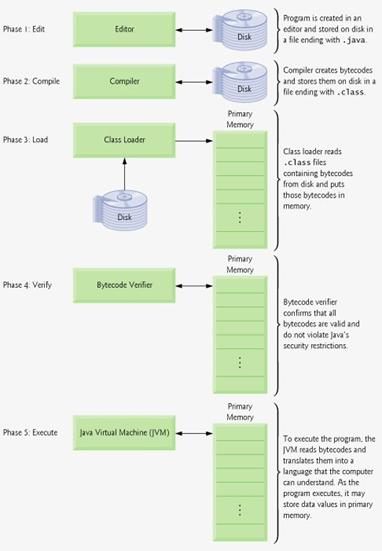
Java has three kinds
of variables (data indentifiers): local
(automatic), instance, and class. Local variables are declared
within a method body. Both instance and class variables are declared inside a
class body but outside of any method bodies. Instance and class variables look
similar, except class variables are prepended with the static modifier.
General Form
Let's take a look at the
general form for declaring each kind of variable in a Java class. The following
class is not real Java code; it is only pseudocode:
class someClass
Variable
identifiers
The
pseudocode above contains three variable declarations. The variable names are instanceVariableName,
classVariableName, and localVariableName. Variable names must be legal Java
identifiers.
Keywords
and reserved words may not be used.
It must
start with a letter, dollar sign ($), or underscore (_).
It is case sensitive. For example,
mytest and MyTest are different identifiers.
Variable scope
Each of the three kinds of variables has a different scope. A
variable's scope defines how long that variable lives in the program's memory
and when it expires. Once a variable goes out of scope, its memory space is
marked for garbage collection by the JVM and the variable may no longer be
referenced.
Notice that both instanceVariableName and classVariableName are
declared within someClass but outside of any of its methods (only one method
exists in this example). localVariableName, on the other hand, is declared
within someMethod. Local variables must be declared within methods. This
includes being declared within code blocks nested inside of a method--within an
if, while, or for block, for
instance. A variable is local to the code block within which it is declared.
Being declared within a method body makes a variable local to that method.
Being declared within an if block makes the variable local to that if block,
for example. This means that the variable cannot be used outside of the curly
braces within which it was declared. In fact, it can only be used from the line
it is declared on until the code block ends.
Variable
type
Each of the three variables in our general form example also has a
variable_type modifier. variable_type defines the type of data that the
variable holds. It must be either a Java primitive (int, boolean, etc.) or a
Java class (String, Object, MyTest, etc.
Object
references are variables that refer to Java objects. Instead of holding a
value, they hold the memory address of the object. The object may be of a
user-defined class or it may be one of the classes included in the Java APIs
such as java.lang.String or java.util.List.
Here are all the
possible variable types with their memory requirement and default values:
|
Java
Variables
|
|
Type
|
Size
in Bits
|
Initialization
|
|
boolean
|
|
false
|
|
char
|
|
'uoooo'
|
|
byte
|
|
|
|
short
|
|
|
|
int
|
|
|
|
long
|
|
0L
|
|
float
|
|
0.0F
|
|
double
|
|
|
Variable visibility
The visibility (also
know as access scope) of instance
and class variables defines what objects can read and modify that variable. The
four possible visibility modifiers are: public,
protected, private, and no modifier.
If no visibility modifier is included with an instance or class variable, then
it is said to have default visibility. Keeping an object's data hidden is
called encapsulation and is one of the tenents of good object-oriented
development.
|
Variable
Visibility
|
|
Modifier
|
Can
be Accessed By
|
|
public
|
any class
|
|
protected
|
owning class, any subclass, any class in the same
package
|
|
no modifier
|
owning class, any class in the same package
|
|
private
|
owning class
|
A graphical
user interface (GUI) presents a user-friendly mechanism for interacting
with an application . GUIs are built from GUI
components. These are sometimes called controls or widgets
short for window
gadgets in other languages . Below we list several swing components
that we used to create our GUI
3.2 Packages used for the application
from Java
javax.swing.JFrame
- this class implements accessibility support for the JFrame class
javax.swing.JButton
- an implementation of a 'push' button.
javax.swing.JMenu
- an implementation of a menu -- a popup window
containing JMenuItems that is displayed when the user selects an item on the JMenuBar
javax.swing.JMenuBar
- an implementation of a menu bar. You add JMenu objects to
the menu bar to construct a menu
javax.swing.JMenuItem
- an implementation of an item in a menu. A menu item
is essentially a button sitting in a list. When the user selects the
'button', the action associated with the menu item is performed.
javax.swing.Icon
- a small fixed size picture, typically used to
decorate components.
javax.swing.ImageIcon
- a small fixed size picture, typically used to
decorate components. Methods here: getIconHeight ,
getIconWidth() and paintIcon which paints the icon at a
specified locations
javax.swing.SwingConstants - a
collection of constants generally used for positioning and orienting components
on the screen.
Options :
bottom - Box-orientation constant used to specify the bottom of a box
center - The central position in an area.
east - Compass-direction east (right).
horizontal - Horizontal orientation.
leading - Identifies the leading edge of text
for use with left-to-right and right-to-left languages
left - Box-orientation constant used to
specify the left side of a box.
north - Compass-direction North (up).
north east - Compass-direction
north-east (upper right).
north west - Compass-direction north west
(upper left).
right - Box-orientation constant used to
specify the right side of a box.
south - Compass-direction south (down).
south east - Compass-direction south-east
(lower right).
south west - Compass-direction south-east
(lower right).
top - Box-orientation constant used to specify
the top of a box.
vertical - Vertical orientation.
west - Compass-direction west (left).
javax.swing.JCheckBoxMenuItem
- a menu item that can be selected or deselected. If
selected, the menu item typically appears with a checkmark next to it. If
unselected or deselected, the menu item appears without a checkmark. Like a
regular menu item, a check box menu item can have either text or a graphic icon
associated with it, or both. Either isSelected/setSelected
or getState/setState
can be used to determine/specify the menu item's selection state. The
preferred methods are isSelected
and setSelected,
which work for all menus and buttons. The getState and setState
methods exist for compatibility with other component sets.
javax.swing.JPanel
- a generic lightweight container. If no options
specified it creates a JPanel with a double buffer and a flow layout.
javax.swing.JscrollPane
- provides a scrollable view of a lightweight
component. A JscrollPane manages a viewport, optional vertical and horizontal
scroll bars, and optional row and column heading viewports.
javax.swing.JTextArea
- is a multi-line area that displays plain text. It is
intended to be a lightweight component that provides source compatibility with
the awt.TextArea
javax.swing.JToolBar
- provides a component that is useful for displaying
commonly used actions or controls
There are actually
two sets of GUI components in Java. Before Swing was introduced in J2SE 1.2,
Java GUIs were built with components from the Abstract
Window Toolkit (AWT) in package java.awt.
When a Java application with an AWT GUI executes on different Java platforms,
the application's GUI components display differently on each platform. Here are
the awt components that I used.
java.awt.BorderLayout -
a border layout lays out a container, arranging and
resizing its components to fit in five regions: north, south, east, west, and
center. Each region may contain no more than one component, and is identified
by a corresponding constant: NORTH SOUTH EAST WEST, and CENTER. When adding a component to a container with a border layout, use one
of these five constants, for example:
Panel p = new Panel();
p.setLayout(new BorderLayout());
p.add(new Button('Okay'), BorderLayout.SOUTH);
java.awt.Dimension
- this class encapsulates the width and height of a
component (in integer precision) in a single object. The class is associated
with certain properties of components.
java.awt.FileDialog
- displays a dialog window from which the user can
select a file.
java.awt.FlowLayout
- a flow layout arranges components in a left-to-right
flow, much like lines of text in a paragraph. Flow layouts are typically used
to arrange buttons in a panel. It will arrange buttons left to right until no
more buttons fit on the same line. Each line is centered.
import java.awt.*; import java.applet.Applet; public class myButtons extends Applet
This is the code for the flowlayout
java.awt.Frame
- a Frame is a top-level window with a title and a
border . The size of the frame includes any area designated for the border. The
dimensions of the border area may be obtained using the getInsets method,
however, since these dimensions are platform-dependent, a valid insets value
cannot be obtained until the frame is made displayable by either calling pack or show. Since the
border area is included in the overall size of the frame, the border
effectively obscures a portion of the frame, constraining the area available
for rendering and/or displaying subcomponents to the rectangle which has an
upper-left corner location of (insets.left,
insets.top), and has a size of width - (insets.left + insets.right) by height -
(insets.top + insets.bottom). Frames are capable of
generating the following types of WindowEvents:
WINDOW_OPENED
WINDOW_CLOSING
WINDOW_CLOSED
WINDOW_ICONIFIED
WINDOW_DEICONIFIED
WINDOW_ACTIVATED
WINDOW_DEACTIVATED
WINDOW_GAINED_FOCUS
WINDOW_LOST_FOCUS
WINDOW_STATE_CHANGED
java.awt.Graphics - The class is
the abstract base class for all graphics contexts that allow an application to
draw onto components that are realized on various devices, as well as onto
off-screen images.
java.awt.Graphics2D
- extends the Graphics class to provide more
sophisticated control over geometry, coordinate transformations, color
management, and text layout. This is the fundamental class for rendering
2-dimensional shapes, text and images on the Java(tm) platform
java.awt.GridBagConstraints
- specifies constraints for components that are laid
out using the GridBagLayout class
java.awt.GridBagLayout
- a flexible layout manager that aligns components
vertically and horizontally, without requiring that the components be of the
same size. Each GridBagLayout object maintains a dynamic, rectangular grid of cells, with each
component occupying one or more cells, called its display area.
Values:
GridBagConstraints.NORTH
GridBagConstraints.SOUTH
GridBagConstraints.WEST
GridBagConstraints.EAST
GridBagConstraints.NORTHWEST
GridBagConstraints.NORTHEAST
GridBagConstraints.SOUTHWEST
java.awt.Insets
- a representation of the borders of a container. It
specifies the space that a container must leave at each of its edges. The space
can be a border, a blank space, or a title. Can be : bottom , left, right , top
java.awt.Label
- component for placing text in a container. A label
displays a single line of read-only text. The text can be changed by the
application, but a user cannot edit it directly.
java.awt.TextField
- text component that allows for the editing of a
single line of text.
java.awt.event.ActionEvent
- event which indicates that a component-defined
action occured. This high-level event is generated by a component (such as a
Button) when the component-specific action occurs (such as being pressed). The
event is passed to every every ActionListener object that registered to
receive such events using the component's addActionListener method.
java.awt.event.ActionListener
- the event which indicates that a component-defined
action occured. This high-level event is generated by a component (such as a
Button) when the component-specific action occurs (such as being pressed). The
event is passed to every every ActionListener object that registered to
receive such events using the component's addActionListener method.
The actions invoked when event occures actionPerformed(ActionEvent e)
java.awt.event.WindowAdapter
- an abstract adapter class for receiving window
events. The methods in this class are empty. This class exists as convenience
for creating listener objects.
java.awt.event.WindowEvent
- a low-level event that indicates that a window has
changed its status. This low-level event is generated by a Window object when
it is opened, closed, activated, deactivated, iconified, or deiconified, or
when focus is transfered into or out of the Window.
java.awt.event.InputEvent
- the root event class for all component-level input
events. Input events are delivered to listeners before they are processed
normally by the source where they originated. This allows listeners and
component subclasses to 'consume' the event so that the source will
not process them in their default manner. For example, consuming mousePressed
events on a Button component will prevent the Button from being activated.
java.awt.event.MouseEvent
- is an event which indicates that a mouse action
occurred in a component. A mouse action is considered to occur in a particular
component if and only if the mouse cursor is over the unobscured part of the
component's bounds when the action happens. Component bounds can be obscurred
by the visible component's children or by a menu or by a top-level window. This
event is used both for mouse events (click, enter, exit) and mouse motion
events (moves and drags).
This low-level event is generated by a
component object for:
- Mouse Events
- a mouse button is pressed
- a mouse button is released
- a mouse button is clicked (pressed and released)
- the mouse cursor enters the unobscured part of
component's geometry
- the mouse cursor exits the unobscured part of
component's geometry
- Mouse Motion Events
- the mouse is moved
- the mouse is dragged
java.awt.event.MouseMotionAdapter
- abstract adapter class for receiving mouse motion
events. The methods in this class are empty. This class exists as convenience
for creating listener objects. Mouse motion events occur when a mouse is moved
or dragged. (Many such events will be generated in a normal program. To track
clicks and other mouse events, use the MouseAdapter.)
java.awt.geom.Arc2D
- Arc2D is the abstract superclass for all objects that store a 2D arc defined
by a bounding rectangle, start angle, angular extent (length of the arc), and a
closure type (OPEN CHORD, or PIE
java.awt.geom.CubicCurve2D
- the CubicCurve2D class defines a cubic
parametric curve segment in (x, y) coordinate space.
java.awt.geom.Line2D
- represents a line segment in (x, y) coordinate
space. This class, like all of the Java 2D API, uses a default coordinate
system called user space in which the y-axis values increase downward
and x-axis values increase to the right
java.awt.geom.QuadCurve2D
- defines a quadratic parametric curve segment in
(x, y) coordinate space.
java.awt.geom.RoundRectangle2D
- defines a rectangle with rounded corners defined by
a location (x, y), a dimension (w x h), and the width and height
of an arc with which to round the corners.
java.io.BufferedInputStream
- adds functionality to another input stream-namely,
the ability to buffer the input and to support the mark and reset methods.
When the BufferedInputStream is created, an internal buffer array is created. As bytes from the
stream are read or skipped, the internal buffer is refilled as necessary from
the contained input stream, many bytes at a time. The mark operation remembers
a point in the input stream and the reset operation causes all
the bytes read since the most recent mark operation to be
reread before new bytes are taken from the contained input stream.
java.io.BufferedOutputStream
- implements a buffered output stream. By setting up
such an output stream, an application can write bytes to the underlying output
stream without necessarily causing a call to the underlying system for each
byte written.
java.io.DataInputStream
- lets an application read primitive Java data types
from an underlying input stream in a machine-independent way. An application
uses a data output stream to write data that can later be read by a data input
stream. Data input streams and data
output streams represent Unicode strings in a format that is a slight
modification of UTF-8.
java.io.DataOutputStream
- lets an application write primitive Java data types
to an output stream in a portable way. An application can then use a data input
stream to read the data back in.
java.io.FileInputStream
- obtains input bytes from a file in a file system.
What files are available depends on the host environment.
java.io.FileOutputStream
- A file output stream is an output stream for writing
data to a File or to a FileDescriptor. Whether or not a file is available or may be created depends upon the
underlying platform. Some platforms, in particular, allow a file to be opened
for writing by only one FileOutputStream (or other file-writing object) at a time. In such situations the
constructors in this class will fail if the file involved is already open.
java.io.IOException
- signals that an I/O exception of some sort has
occurred. This class is the general class of exceptions produced by failed or
interrupted I/O operations.
java.io.ObjectInputStream
- provide an application with persistent storage for
graphs of objects when used with a FileOutputStream and FileInputStream
respectively. Ensures that the types of all objects in the graph created from
the stream match the classes present in the Java Virtual Machine. Classes are
loaded as required using the standard mechanisms. The method readObject is used
to read an object from the stream. Java's safe casting should be used to get
the desired type. In Java, strings and arrays are objects and are treated as objects.
java.io.ObjectOutputStream
- writes primitive data types and graphs of Java
objects to an OutputStream. The objects can be read (reconstituted) using an
ObjectInputStream. Persistent storage of objects can be accomplished by using a
file for the stream. If the stream is a network socket stream, the objects can
be reconsituted on another host or in another process. The method writeObject is used to write an object to the stream. Any object, including
Strings and arrays, is written with writeObject. Multiple objects
or primitives can be written to the stream. The objects must be read back from
the corresponding ObjectInputstream with the same types and in the same order
as they were written.
3.3 Chart2d
Chart2D is a library written in Java for adding
2D charts to Java programs (or for exporting them to images). The goal of library is to provide common chart
types and features for general applications. There are three basic chart
types: LBChart2D, LLChart2D, and PieChart2D. They all share a common configuration
process.
There are two types of objects that need configuration properties
objects and graphical objects. Properties objects are objects that hold
all the settings and information needed by a graphical object to determine how
it should look. Graphical objects are the objects that are added to GUI's
or that export BufferedImage objects of themselves. Properties are
separated from graphical objects because many graphical objects share common
properties .
We want to use PieChart
The PieChart2D object requires the configuration of six properties
objects: Object2DProperties, Chart2DProperties, PieChart2DProperties, LegendProperties,
Dataset, and MultiColorsProperties.
The Object2DProperties object contains seventeen settings for the
object border, background, title, and gaps. The
actual configuration of an Object2DProperties object looks like this.
Methods:
setObjectBorderColor
(java.awt.Color) Sets the color of the object's border. setObjectTitleFontColor
(java.awt.Color) Sets the color of the font for the object's title. setObjectTitleText
(java.lang.String) Sets the text for the object's title.
The actual configuration of an Object2DProperties object looks like
this.:
Object2DProperties
object2DProps = new Object2DProperties();
object2DProps.setObjectTitleText ('Title for this Object');
The next properties object to
configure is a Chart2DProperties object. There are only three settings to
this object. There are only two things that this object manages:
the gap between the legend and the
rest of the chart and
something called 'the data
labels precision'. The data labels precision setting is a complex
one. But basically it adjusts how the labels look
Using the
defaults, the configuration of a Chart2DProperties object looks like this.
Chart2DProperties
chart2DProps = new Chart2DProperties();
The next
properties object to configure is a LegendProperties object. There are
twenty-two settings customizing the legend border, labels, label bullets,
and gaps. Here is a basic graphic of the managed components. The
graphic depicts an area that fits within the legend area managed by the
Chart2DProperties object.
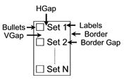
For a pie with 'n' sectors, one needs a Dataset object with
'n' sets, and one also needs a MultiColorsProperties
object with 'n' custom colors For the PieChart2DProperties object, there are twenty-four settings
customizing the pie sectors, pie labels, and pie sector labels lines, and
gaps. Here is a basic graphic of the managed components. The
graphic depicts an area that fits within the chart area managed by the Chart2DProperties object.
The actual
configuration of a GraphChart2DProperties looks like this.
PieChart2DProperties
pieChart2DProps = new PieChart2DProperties();
pieChart2DProps.setPieLabelsFontColor (new Color (000,027,090));
pieChart2DProps.setPieLabelsLinesColor (new Color (000,035,115));
pieChart2DProps.setPieLabelsLinesDotsColor (new Color (000,035,115));
After having configured all
the necessary properties objects, a PieChart2D object must be created and
configured
PieChart2D pieChart2D = new
PieChart2D();
pieChart2D.setObject2DProperties (object2DProps);
pieChart2D.setChart2DProperties (chart2DProps);
pieChart2D.setLegendProperties (legendProps);
pieChart2D.setPieChart2DProperties (pieChart2DProps);
pieChart2D.addDataset (dataset);
pieChart2D.addMultiColorsProperties (multiColorsProps);
3.4
The eclipse platform
Eclipse is a Java-based, extensible open source development platform.
By itself, it is simply a framework and a set of services for building a
development environment from plug-in components. Fortunately, Eclipse comes
with a standard set of plug-ins, including the Java Development Tools (JDT).
Eclipse also includes the Plug-in Development Environment (PDE) which allows developers to create their own
plugins.
Eclipse
is written in the Java language, its use isn't limited to the Java language.
For example, plug-ins are available or planned that include support for
programming languages like C/C++ and COBOL. The Eclipse framework can also be used
as the basis for other types of applications unrelated to software development,
such as content management systems.
The JDT, however, is an addition to Eclipse. At the most
fundamental level, Eclipse is the Eclipse Platform The Eclipse Platform's purpose is
to provide the services necessary for integrating software development tools,
which are implemented as Eclipse plug-ins. To be useful, the Platform has to
be extended with plug-ins such as the JDT.
If you only want to use Eclipse for C/C++ development, then
replace the JDT with the C Development Toolkit (CDT).
The primary job of the Platform runtime is to discover what plug-ins are
available in the Eclipse plug-in directory. Each plug-in has an XML manifest
file that lists the connections the plug-in requires. These include the
extension points it provides to other plug-ins, and the extension points from
other plug-ins that it requires. Because the number of plug-ins is potentially
large, plug-ins are not loaded until they are actually required, to minimize
start-up time and resource requirements.
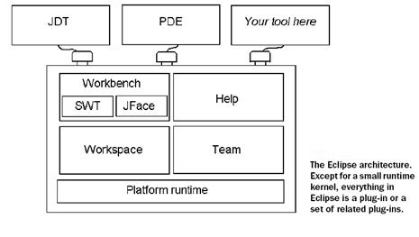
The first step toward getting
started with Eclipse is to download the software from the Eclipse.org web
site's download page at https://www.eclipse.org/ downloads. Here you'll
find the latest and the greatest versions-which are not usually the same things-as well as older
versions of Eclipse.
The first time you
open Eclipse, you see the welcome screen.
Second you will see the workspace
which is responsible for managing the user's resources. They are organized into
one or more projects at the top level. Each project corresponds to a
subdirectory of Eclipse's workspace directory. Each project can contain files
and folders; normally each folder corresponds to a subdirectory of the project
directory, but a folder can also be linked to a directory anywhere in the
filesystem. The workspace maintains a low-level history of changes to each
resource. This makes it possible to undo changes immediately, as well as revert
to a previously saved state-possibly days old, depending on how the user has
configured the history settings. This history also minimizes the risk of losing
resources.
The workspace is also responsible
for notifying interested tools about changes
to the workspace resources. Tools have the ability to tag
projects with a project nature-as a Java project, for example-and can
provide code to configure the project's resources as necessary.
3.4.1 Creating a java project
To create a new Java project, follow these steps:
Right-click in the
Navigator view to bring up a context menu and select New - Project and then choose Java
project
Click Next to start
the New Java Project Wizard
Give a name to your project. Here it is jhtb .
Click Finish.
3.4.2 Adding classes
Once the project is created we need to add the class files and modify
the class path in order to use Chart2D. For adding classes :
Right click in the Package
explorer then New -> Class
Now
we need to add the class path to Chart2d. If we don't we can't get JHTB
working. JHTB is the name of my
project. For modifing class paths we
right click on the project and Properties
then we go to Java build path . We
add class folder
3.4.3 Compiling
After
finishing this steps we compile the
project by going under Run -> Run As
-> Java Application. We should
get the something like below:
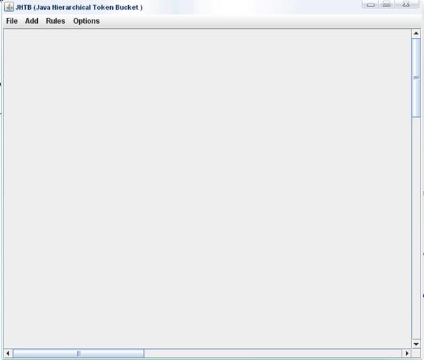
Chapter 4
4.1 The application
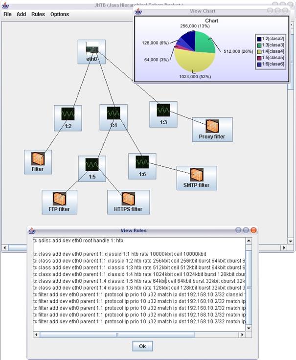
The
goal of this application is to simplify the work using HTB in linux. With this
application you can simply build rules for your home network and develop the
QoS that you need. I will explain in short what this application can do . I
will detaliate this in this chapter.
First
of all you will need to add a network card and set the values which you will
operate later. After doing this you can add classes and play with the filters.
You can generate the rules , save them and even apply them. You can apply them
only if you are on linux. On windows this will thrown an exception in java just
because windows doesn't have the tc binary for running what you have created.
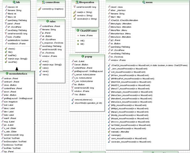
Class diagram - detailed class diagram in
the attachement
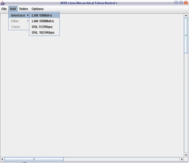
The
code that creates this GUI is the following:
// Main panel
final static JPanel pane1 new JPanel()
// creates
the object
When
inserting the interface we are promted for setting up the rate and the ceil of the
interface.
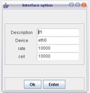
The code is found
on mouseInterface.java. The most important code is below:
public class mouseInterface
extends JFrame
and
public String
generate()
return rule
Next is how to adding a class :
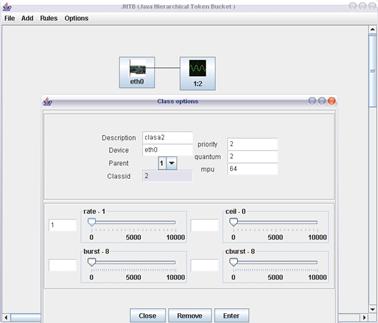
Here the device is automatically
filled and the rates burst ceil and cburst are taken from the upper class
mouseinterface. One example for filling
this class option is :
rate -
256
ceil -
256
burst
- 16
cburst -
16
4.2 Code explication
I
will explain the code that i find interesting. The class is mouseClass.java
//check available rate for the class
int p_rate=0;
int p_ceil_rate=0;
int p_num = menu.clasa1[nr].parent; // we get the
parent number
int min=0; // the
minimum available rate
if(p_num==1)
p_rate=menu.ether rate //if the
parrent is 1 this means the rate of the class is equal with the rate of the
card, in our example is 10000.
else
p_ceil_rate=p_rate;
//the ceil rate = rate of class again
for int i=2;i<=htb.classes;i++)
// no parent class is child
if(p_rate<0)
p_rate=0; // p_rate cannot be negative
for int i=2;i<=htb.classes;i++) //check for children of the class
}
}
After
adding the classes the commands are automatically generated : the code which
generates the tc commands is found in
generatehtb.java
public String generate()
When
we finished adding classes we have to add filters for the classes.
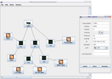
There are to main
types of filters filters
When no port is specified
filter without port information
@param int lx X position for Button
int ly Y position for Button
String ldescr class description
String ldev Device (ex.eth0)
int lparent parent class
int lclassid CLASSID parameter for HTB
String lprotocol defines protocol (only IP)
int lprio queueing priority
String ldirection defines direction can be 'src' or 'dst' for u32 filter
String l_ip defines IP address(es)
String lpdirection port direction
int lfilterid FilterID (for removing)
public filter(int lx,int ly,String
ldescr,String ldev,int lparent,int
lclassid,String lprotocol,
int lprio,String
ldirection,String l_ip,int lfilterid)
When port is specified
filter with port information
@param int lx X position for Button
int ly Y position for Button
String ldescr class description
String ldev Device (ex.eth0)
int lparent parent class
int lclassid CLASSID parameter for HTB
String lprotocol defines protocol (only IP)
int lprio queueing priority
String ldirection defines direction can be 'src' or 'dst' for u32 filter
String l_ip defines IP address(es)
int lport Port
String lpdirection port direction
int lfilterid FilterID (for removing)
@see Serialization
public filter(int lx,int ly,String
ldescr,String ldev,int lparent,int
lclassid,String lprotocol,
int lprio,String
ldirection,String l_ip,int lport,String
lpdirection,int lfilterid)
After we finished
adding the rules we can:
Apply them
static void exec()
}
}catch (IOException ex)
}
Save them to a file - plain text
static void save() catch(IOException ex)
View them
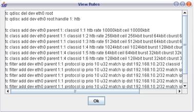
static void view()
catch(NullPointerException
e) ;
sP new JScrollPane(tA
sP.setPreferredSize(new Dimension(520,
240));
jp.add(sP
jp.add(ok ok = button
window.setSize(new Dimension(550,
320));
window.getContentPane().add(jp
window.setResizable(false
///Export
button listener
final
java.awt.event.ActionListener ff2 = new ActionListener()
};
ok.addActionListener(ff2);
// for the button work we must add an action on it
window.setVisible(true
Or save them for loading and
modifing . we use serialization to save all classes (clasa1/filter1/ether) and some
initialization methods.
public static void save(String s)
throws IOException
for int x=2;x<htb.filters;x++)
//load
public static void loadFile()
catch(IOException
ex)
catch
(NullPointerException qq)
At the final we can see our rules
and how is the bandwidht allocated
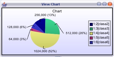
public void init() else
}
legendProps.setLegendLabelsTexts
(legendLabels);
//Configure dataset
int numSets = htb.classes-2, numCats =
1, numItems = 1;
Dataset dataset = new Dataset
(numSets, numCats, numItems);
// Enter data
to graph
for int x=0;x<htb.classes-2;x++)
else
}
//Configure graph component colors
MultiColorsProperties multiColorsProps = new
MultiColorsProperties();
//Configure pie area
PieChart2DProperties pieChart2DProps = new
PieChart2DProperties();
//Configure chart
PieChart2D chart2D = new PieChart2D();
chart2D.setObject2DProperties
(object2DProps);
chart2D.setChart2DProperties
(chart2DProps);
chart2D.setLegendProperties (legendProps);
chart2D.setDataset (dataset);
chart2D.setMultiColorsProperties
(multiColorsProps);
chart2D.setPieChart2DProperties
(pieChart2DProps);
//Optional validation: Prints debug messages if invalid only.
if
(!chart2D.validate (false)) chart2D.validate (true
frame new JFrame();
frame.getContentPane().add
(chart2D); //Add Chart2D to GUI
frame.setTitle ('View
Chart'
frame.addWindowListener (
new WindowAdapter() } );
frame.pack();
Dimension screenSize = Toolkit.getDefaultToolkit().getScreenSize();
frame.setLocation (
(screenSize.width frame.getSize().width
(screenSize.height frame.getSize().height
frame.setVisible(true
}
Bibliography
[TMM03] Core
java data objects , by Sameer Tyagi, Michael Vorburger, Keiron McCammon, and
Heiko Bobzin 2003
[TSH04]
End-to-End QoS Network Design : Quality of Service in LANs , WANs, and
VPNs by Tim Szigeti, Christina Hattingh
2004
[AST02] Computer Networks , Fourth Edditon by
Andrew S. Tanenbaum 2002
[LGH06] Designing
and implementing Linux Firewalls and QoS using netfilter, iproute2, NAT and
L7-filter by Lucian Gheorghe 2006
[HDD04] Java
How to Program (6th Edition) by Harvey
M. Deitel, Paul J. Deitel 2004
[TSK06] Network Administrator Street Smarts: A
Real World Guide to CompTIA Network+ Skills by Toby Skandier 2006
[SST03] Network
Tutorial, Fifth Edition by Steve Steinke 2003
[GBM03] Eclipse in action by David Gallardo, Ed
Burnette, and Robert McGovern 2003
[NMW04] SWT : The Standard Widget Toolkit By Steve Northover, Mike Wilson
2004
[ALS06] QoS for IP/MPLS
Networks By Santiago Alvarez, 2006
[W1] Kernel
Parameters
https://lartc.org/howto/lartc.kernel.obscure.html
[W2] Linux
Traffic control
https://linux-ip.net/articles/Traffic-Control-HOWTO/index.html
[W3] Practical Guide to Linux Traffic Control
https://www.trekweb.com/~jasonb/articles/traffic_shaping/index.html
[W4] HTB tools webpage
https://htb-tools.arny.ro/content.php
[W5] HTB Manual
https://luxik.cdi.cz/~devik/qos/htb/manual/userg.htm
[W6] Ipsysctl tutorial
https://ipsysctl-tutorial.frozentux.net/ipsysctl-tutorial.html
[W7] Traffic Shaping with Linux v2.4 and HTB qdisc
https://www.trekweb.com/~jasonb/articles/linux_tc_minihowto.shtml
[W8] Module that extends iptables to match peer-to-peer
(P2P) data in IP traffic
https://www.ipp2p.org/
[W9] Packet filtering on linux
https://www.netfilter.org
[W10] Online encyclopedia / dictionary
https://www.wikipedia.org/
and https://www.webopedia.com/